RSYC
Remote Sensing-Derived Yield Curves for Canada
Provides published remote sensing-based yield curves for
aboveground biomass and total volume across Canada, as described in
Tompalski et al. (2024)
RSYC: Remote Sensing-Based Yield Curves for Canada

RSYC provides published yield curves for aboveground biomass (AGB,
Mg/ha) and total volume (m3/ha). Curves are available for individual
species and the generic, coniferous, and broadleaf model groups.
Models are available for 150 x 150 km tiles and four nested ecological levels: ecozone, ecoprovince, ecoregion, and ecodistrict.
Models are periodically updated as new remote sensing data become available. The current release is v20260923.
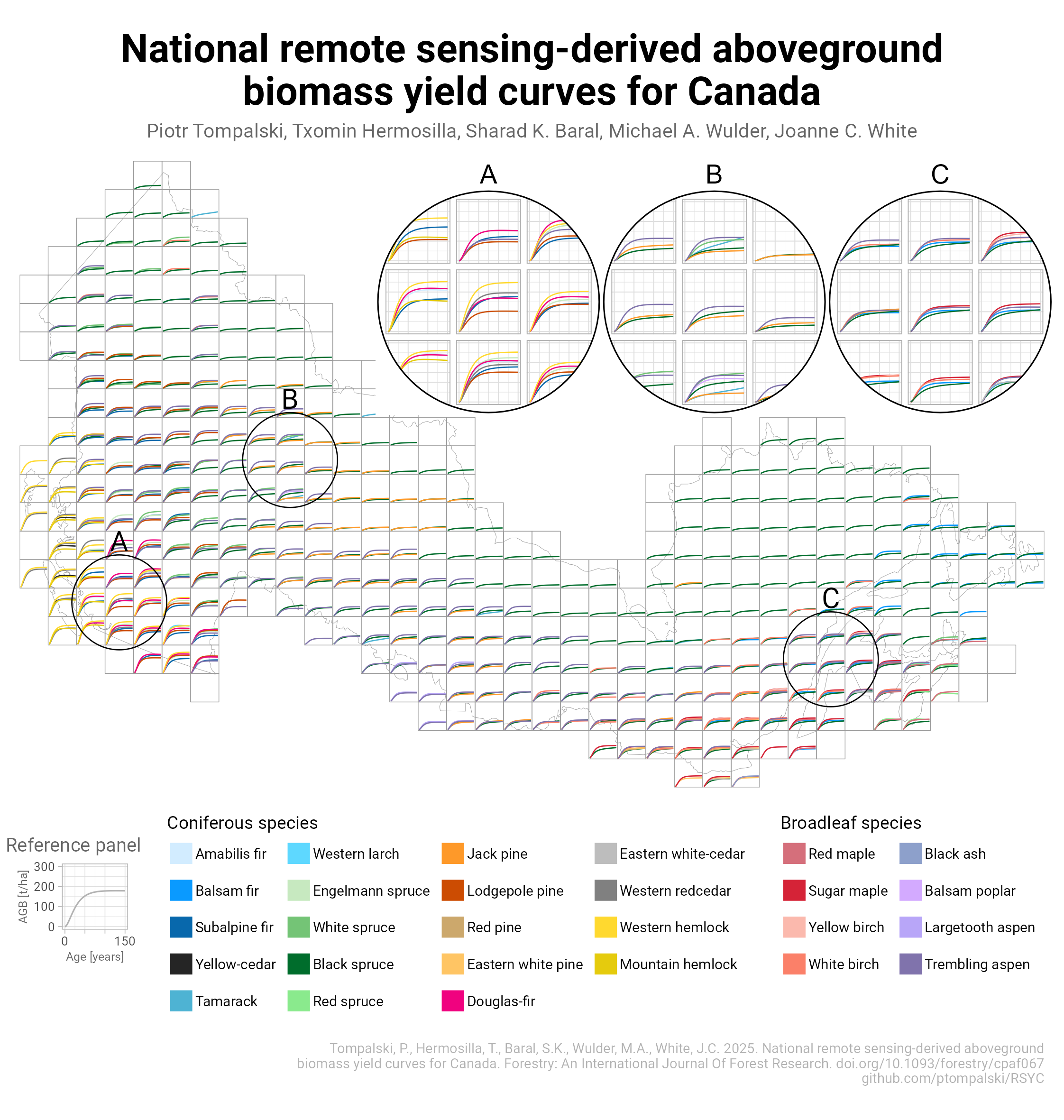 Species-specific RSYC curves across
Canada’s 150 km tile grid.
Model parameters
You don’t need to install the R package to use the models. All model
parameters used in RSYC are available for direct download. The ZIP
archive contains the updated RSYC_models.csv table, including AGB and
volume models for tiles and ecological strata.
-
Model parameters: RSYC_models.zip
-
Tile grid: RSYC_tiles.gpkg
-
Ecological strata: RSYC_ecostrat.gpkg
The RSYC models predict aboveground biomass (AGB) or total volume as a function of stand age:
$$ y = b_1 e^{-b_4 \mathrm{Age}} (1 - e^{-b_2 \mathrm{Age}})^{b_3}. $$
where
- $y$ is AGB (Mg/ha) or total volume (m3/ha)
- $b_1, b_2, b_3, b_4$ are response-, stratum-, and species-specific parameters
- Age is stand age (years)
The curves were fitted for stand ages 1 to 150 years. RSYC warns when asked to estimate outside this age range.
Installation
# install.packages("remotes")
# Development version with model release v20260923:
remotes::install_github("ptompalski/RSYC", ref = "dev")
Examples
Estimate biomass or volume
Estimate AGB for black spruce (PICE.MAR) in tile H14 at stand ages 20,
60, and 120 years:
library(RSYC)
predict_rsyc("agb", "PICE.MAR", c(20, 60, 120), "tile", "H14")
#> [1] 26.85001 58.32616 71.92139
To estimate total volume instead, set response = "volume":
predict_rsyc(
  response = "volume",
  species = "PICE.MAR",
  age = c(20, 60, 120),
  strata_level = "tile",
  strata_id = "H14"
)
For ecological strata, e.g. ecodistrict “Windsor Lowlands”, use the same function:
predict_rsyc(
  response = "agb",
  species = "PICE.MAR",
  age = c(20, 60, 120),
  strata_level = "ecodistrict",
  strata_id = "Windsor Lowlands"
)
Several species and tiles
The following example estimates AGB and volume for several species,
stand ages, and tiles. Each row of tile_inputs describes one estimate.
tile_inputs <- tidyr::crossing(
  response = c("agb", "volume"),
  species = c("PICE.MAR", "POPU.TRE", "coniferous"),
  age = c(20, 60, 120),
  strata_level = "tile",
  strata_id = c("H14", "F31")
) |>
  dplyr::mutate(
    prediction = purrr::pmap_dbl(
      list(response, species, age, strata_level, strata_id),
      predict_rsyc
    )
  )

tile_inputs
Compare ecological levels
Use the area name at the chosen ecological level when that name occurs only once.
eco_inputs <- tibble::tribble(
  ~response, ~species,   ~age, ~strata_level, ~strata_id,
  "agb",     "PICE.MAR", 80,  "ecozone",
    "Atlantic Maritime",
  "agb",     "PICE.MAR", 80,  "ecoprovince",
    "Appalachian-Acadian Highlands",
  "agb",     "PICE.MAR", 80,  "ecoregion",
    "Appalachians",
  "agb",     "PICE.MAR", 80,  "ecodistrict",
    "Windsor Lowlands"
)

eco_inputs <- eco_inputs |>
  dplyr::mutate(
    prediction = purrr::pmap_dbl(
      list(response, species, age, strata_level, strata_id),
      predict_rsyc
    )
  )

eco_inputs
The same species can have different curves at each nested ecological level. The example below shows black spruce volume curves together with the areas they represent:
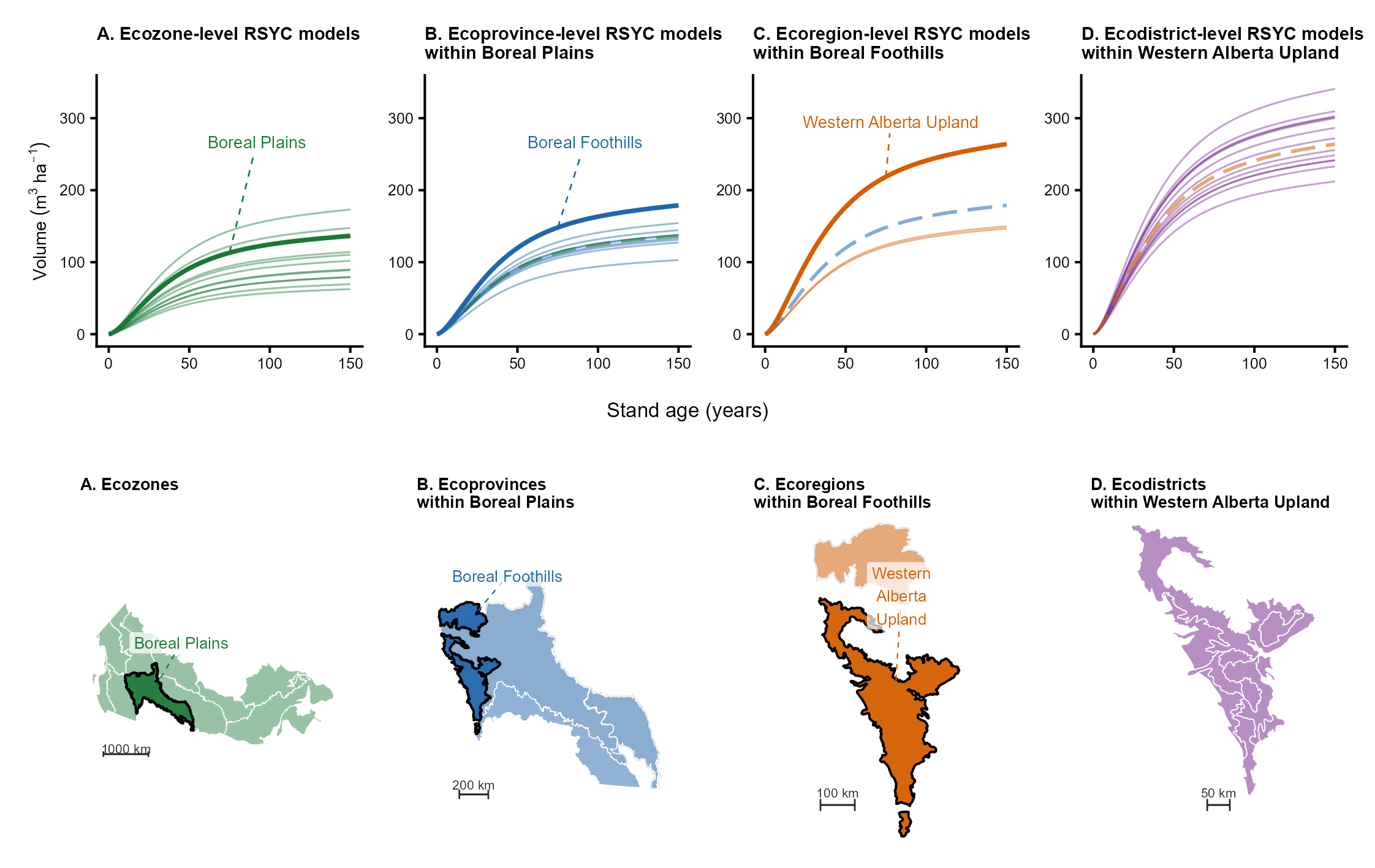 Black spruce volume curves and maps at
four nested ecological levels.
Generate several complete curves
The following example produces a complete set of estimates for ages 1 to
150 for each species and area listed in curve_inputs:
curve_inputs <- tibble::tribble(
  ~response, ~species,    ~strata_level, ~strata_id,
  "agb",     "PICE.MAR",  "tile",       "H14",
  "agb",     "POPU.TRE",  "tile",       "F31",
  "volume",  "coniferous", "tile",       "N3"
)
curve_inputs <- curve_inputs |>
  dplyr::mutate(
    age = list(1:150),
    prediction = purrr::pmap(
      list(response, species, age, strata_level, strata_id),
      predict_rsyc
    )
  )

curve_inputs
#> # A tibble: 3 × 6
#>   response species    strata_level strata_id age         prediction
#>   <chr>    <chr>      <chr>        <chr>     <list>      <list>
#> 1 agb      PICE.MAR   tile         H14       <int [150]> <dbl [150]>
#> 2 agb      POPU.TRE   tile         F31       <int [150]> <dbl [150]>
#> 3 volume   coniferous tile         N3        <int [150]> <dbl [150]>

curve_predictions <- curve_inputs |>
  tidyr::unnest(c(age, prediction))
Plot the curves to compare how predicted yield changes with stand age. AGB and volume are shown separately because they use different units:
curve_predictions |>
  dplyr::mutate(
    response = factor(
      response,
      levels = c("agb", "volume"),
      labels = c("AGB (Mg/ha)", "Volume (m3/ha)")
    ),
    curve = paste(species, strata_id, sep = " - ")
  ) |>
  ggplot2::ggplot(ggplot2::aes(age, prediction, colour = curve)) +
  ggplot2::geom_line(linewidth = 0.9) +
  ggplot2::facet_wrap(ggplot2::vars(response), scales = "free_y") +
  ggplot2::labs(
    x = "Stand age (years)",
    y = "Predicted yield",
    colour = "Species and tile"
  ) +
  ggplot2::theme_minimal() +
  ggplot2::theme(legend.position = "bottom")
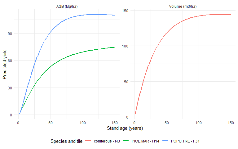
See Prediction examples for a longer walkthrough, including model-availability checks.
Find available curves
Three functions are provided to help identify which model to use:
available_rsyc_models()lists individual published curves that match a response, species, type of area, or area name. For example, list the volume curves for black spruce at the ecozone level:
available_rsyc_models(
  response = "volume",
  species = "PICE.MAR",
  strata_level = "ecozone"
)
rsyc_species()lists the species available for a selected response and area. It also gives each species’ common name and model group. For example, list the AGB species available in tile H14:
rsyc_species(response = "agb", strata_level = "tile", strata_id = "H14")
rsyc_strata()lists the areas for which models are available for a selected response and species. It gives both the short area name and the full hierarchical area identifier, which can distinguish repeated area names. For example, list the ecozones with volume models for black spruce:
rsyc_strata(
  response = "volume",
  species = "PICE.MAR",
  strata_level = "ecozone"
)
Create spatial yield-curve datasets
build_rsyc_dataset() prepares yield estimates and the matching area
boundaries. The boundaries are stored separately so the same map shape
is not repeated for every species and stand age. By default, the
function estimates ages 1 through 150:
dataset <- build_rsyc_dataset(
  response = "volume",
  species = c("PICE.MAR", "POPU.TRE"),
  age = 1:200,
  strata_level = "ecodistrict"
)

dataset$spatial
dataset$curves
dataset$metadata
The spatial map contains strata_id, the ecological area names, and
the area shapes. For tiles, it contains only strata_id and the tile
shapes. The curves table records the model, area, species, stand age,
and estimated yield. The metadata table summarizes the units, model
version, equation, and choices used to create the results.
Use output = "rsyc_volume.gpkg" to save the map, yield curves, and
summary information together in one GeoPackage file.
Presentations and papers
For a visual introduction to the models, start with the RSYC overview. A second presentation, RSYC at IBFRA 2026, focuses on their use in national forest growth and carbon assessment.
If you use the RSYC package in your work, please cite the following two references:
Tompalski, P., Hermosilla, T., Baral, S.K., Wulder, M.A., White, J.C. 2025. National remote sensing-derived aboveground biomass yield curves for Canada. Forestry: An International Journal of Forest Research. https://doi.org/10.1093/forestry/cpaf067
Tompalski, P., Wulder, M.A., White, J.C., Hermosilla, T., Riofrio, J., Kurz, W.A. 2024. Developing aboveground biomass yield curves for dominant boreal tree species from time series remote sensing data. Forest Ecology and Management 561, 121894. https://doi.org/10.1016/j.foreco.2024.121894