linf
L-Infinity Normalization and Dominant Community State Types
Implements L-infinity normalization for compositional matrices,
assigns samples to dominant features, constructs truncated and
hierarchically refined dominant community state types, constructs unordered
dominance sets with support-based sample filtering, and computes
representative landmark profiles. The methods are described by Gajer and
Ravel (2025)


linf: group samples by their most abundant features
linf works with nonnegative measurements, such as microbial counts or proportions. Supply a numeric matrix with samples in rows and features in columns. A feature is a measured quantity, such as the abundance of a type of bacterium.
The package can rescale each sample by its largest value, group samples by which features are most abundant, and divide those groups into smaller groups. It can also assign new samples to groups you have already defined. The groups are called dominant community state types (dCSTs) in the package and methods paper.
A first example
After installation, try this example. n0 = 4 means a
group must initially contain at least four samples to be kept.
set.seed(1) makes the randomly generated example data repeatable.
library(linf)
set.seed(1)
counts <- matrix(rpois(30, 5), nrow = 10,
                 dimnames = list(paste0("s", 1:10), c("A", "B", "C")))
M <- normalize.linf(counts)
dominant <- linf.dominant.features(M)
fit <- linf.csts(M, n0 = 4, low.freq.policy = "absorb")
| Feature | Samples before reassignment | Samples after reassignment |
|---|---|---|
| A | 4 | 6 |
| B | 4 | 4 |
| C | 2 | 0 |
Each sample is first assigned to its largest feature. When largest
values are equal, the first column is used. This gives four samples to
A, four to B, and two to C. Groups A and B meet the minimum size of
four. Group C is too small, so each of its samples is reassigned to A or
B, whichever has the larger value in that sample. Here, both go to A:
the final groups contain six and four samples. The option "absorb"
selects this reassignment rule. A was not the largest feature in the two
reassigned samples; C was.
M contains the rescaled values. Each sample’s largest value is now
one, and zeros stay zero. Use M directly if you only need rescaling,
without groups.
Group by leading features, regardless of their order
Use linf.udcsts() when samples should belong to the same group if they
have the same leading features. For example, A followed by B and B
followed by A both count towards one {A, B} group. The minimum group
size is checked after combining them:
U <- rbind(c(A = 9, B = 5, C = 1), c(A = 8, B = 4, C = 1),
           c(A = 4, B = 9, C = 1), c(A = 3, B = 8, C = 1),
           c(A = 1, B = 3, C = 9))
unordered <- linf.udcsts(U, level = 2, n0 = 3, low.freq.policy = "filter")
unordered$frequency.table
#>    ID freq cumm.pct
#> 1 1,2    4       80
#> 2 2,3    1      100
U[unordered$keep, , drop = FALSE]
#>      A B C
#> [1,] 9 5 1
#> [2,] 8 4 1
#> [3,] 4 9 1
#> [4,] 3 8 1
The four samples led by A and B remain. The single sample led by B and C is excluded because its group is smaller than three. It is not reassigned.
The result includes:
ID: the original column numbers of the features in each group;1,2means A and B here.freq: the number of samples originally in that group, before any reassignment or exclusion.cumm.pct: the percentage of all input samples in this group and groups at least as large. Groups with equal counts get the same percentage. Here the four A/B samples account for 80% of the five input samples.pure.id: the original group of each sample, kept even if it is later reassigned or excluded.
The "filter" option excludes samples from small groups, as above. The
"pure" option keeps them but marks them as rare. The "absorb" option
reassigns them to the kept group whose features have the largest
combined abundance in that sample. This differs from linf.csts(),
which uses one feature at a time and restricts each subdivision to its
current group. See ?linf.udcsts for details.
Connect groups in a network
linf.udcst.graph() connects groups defined by their two leading
features. By default, pairs such as {A, B} and {A, C} are linked
only if both occur among samples whose three leading features are
{A, B, C}. Sharing A alone is not enough.
The result records the supporting sample counts, measures of how often
each pair and its three-feature group occur together, and which group
each sample belongs to. Counts use all input samples, even if you keep
only some pairs in the network. It also reports triangles supported by
the same three-feature group. Every link has length one; a larger sample
count does not shorten it. Unconnected pairs and separate parts of the
network are kept. See ?linf.udcst.graph for details.
Installation
Install the released package from CRAN:
install.packages("linf")
linf.udcsts() and linf.udcst.graph() require linf 0.4.0 or
later. Check your installed version with packageVersion("linf").
Version 0.4.0 includes four guides, called vignettes in R. Open the
function and example-data guides with:
help("linf", package = "linf")
vignette("function-guide", package = "linf")
vignette("example-datasets", package = "linf")
The published website is updated separately and may describe an older version. Use the installed help for the version you run.
Choose the next step
- Prepare the data:
filter.asv()removes samples with too few total counts and features that occur in too few samples.normalize.linf()divides each sample’s values by its largest value. Samples whose largest value is at or below the chosen cutoff (tol) are left unchanged, including all-zero samples. - Form groups:
linf.dominant.features()identifies each sample’s largest feature.linf.csts()forms groups with a minimum size;refine.linf.csts()divides selected groups into smaller groups using their next leading features. - Inspect results:
summary()counts assigned, rare and unassigned samples.linf.landmarks()selects representative samples from the observed data using a chosen feature’s value, for example the sample closest to its mean or median. It returns actual samples, not averages of their measurements. - Assign new samples:
transfer.dcsts()uses the groups defined by an earlier call tolinf.csts(), without changing their definitions.
Scaling by the largest value is called L-infinity normalization. The values are not required to sum to one, and no logarithms are taken. Zeros stay zero. Grouping results depend on which features you include, the minimum group size, how small groups are handled, and how choices between equal values are made. Adding more levels gives finer groups, but does not necessarily make them more useful. The function guide source explains these choices with runnable examples.
Gut microbiome example
The figure below shows the first level of grouping for 766 gut microbiome samples provided with the package, from the American Gut Project (AGP). Filtering leaves 763 samples and 307 microbial features. Groups initially containing fewer than 30 samples are too small to keep. Their samples are reassigned to the kept groups, using the largest value among the remaining defining features in each sample. The figure shows the resulting groups, without a separate rare-sample category.
This subset includes every available sample assigned to four selected uncommon groups. The remaining places were filled by random selection from other eligible samples, using seed 42. Selection did not use participants’ recorded traits. Because groups had different chances of being selected, do not use the observed trait frequencies, differences between groups, or statistical test results to draw conclusions about the broader population. These data are provided to demonstrate how to use the package.
Number of samples in each group
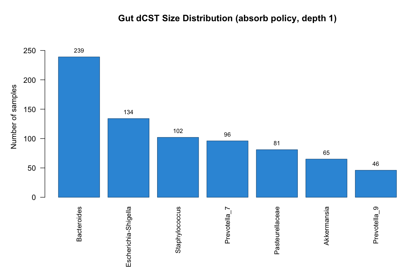
The 763 samples are assigned to seven groups. The largest are Bacteroides (239 samples), Escherichia-Shigella (134), and Staphylococcus (102). In total, 159 samples were reassigned from groups below the minimum size.
See vignette("linf-intro", package = "linf") for a reproducible
example using these data.
Guides and worked examples
Version 0.4.0 includes four installed guides. The first two links below open their source files on GitHub; the R commands open the formatted guides locally.
- Finding your way around linf — choose
functions, arrange your data, handle small groups, select
representative samples, and assign new samples to existing groups.
Open with
vignette("function-guide", package = "linf"). - Example datasets and reproducible
workflows — choose among the five
example datasets, match sample information to data rows, and try
defining groups with one set of samples and assigning another set to
them. Open with
vignette("example-datasets", package = "linf"). - Gut microbiome example — rescale the data, form groups, and explore the selected AGP gut samples.
- Vaginal microbiome example — form groups and compare them with Valencia classifier labels. The samples come from the same source dataset used to develop the classifier; agreement here does not establish performance on independent samples.
The interactive 3D visualization example is available on the website only.
browseVignettes("linf")
Citation
If you use this package, please cite:
Gajer, P. & Ravel, J. (2025). A New Approach to Compositional Data Analysis using L∞-normalization with Applications to Vaginal Microbiome. arXiv preprint arXiv:2503.21543 [stat.CO]. doi: 10.48550/arXiv.2503.21543
BibTeX
@article{gajer2025linf,
  title   = {A New Approach to Compositional Data Analysis using
             {$L^{\infty}$}-normalization with Applications to
             Vaginal Microbiome},
  author  = {Gajer, Pawel and Ravel, Jacques},
  year    = {2025},
  eprint  = {2503.21543},
  archivePrefix = {arXiv},
  primaryClass  = {stat.CO},
  journal = {arXiv preprint arXiv:2503.21543},
  doi     = {10.48550/arXiv.2503.21543},
  url     = {https://arxiv.org/abs/2503.21543}
}
License
MIT © 2025 Pawel Gajer. See LICENSE. Sources and reuse conditions for the example data are recorded in the data-source notes.