ngvb
Latent Non-Gaussian Modelling with 'INLA' and Variational Bayes
Diagnoses whether the latent Gaussian assumption of a model fitted
with the 'INLA' package is adequate, and fits latent non-Gaussian extensions
that relax it. The function ng.check() reports a Bayes-factor sensitivity
diagnostic that says whether, and where, the Gaussian assumption is
inadequate; ngvb() then fits the non-Gaussian model by a variational-Bayes
loop around 'INLA', adding local flexibility only where the data support it.
A single unified engine implements the conditional precision
Q(theta, V) = D(theta)^T diag(1/V) D(theta) and owns its normalizing
constant, and a model registry covers iid, random-walk, autoregressive,
Ornstein-Uhlenbeck, intrinsic-CAR (besag), simultaneous-autoregression,
'SPDE'/Matern and seasonal models. Methods follow Cabral, Bolin and Rue
(2024)
ngvb




Statistical models routinely assume Gaussianity for latent processes (to smooth a signal in space or time, say) largely because it's convenient, not because it's actually appropriate. It's required by many packages such as R-INLA. That assumption is typically left unchecked: is the latent Gaussian assumption reasonable? Is it supported by the data? Which conclusions would change if it were relaxed? And can a more flexible non-Gaussian model even be fit easily?
ngvb (non-Gaussian variational Bayes) answers these questions for R-INLA. It takes an ordinary R-INLA latent Gaussian model (LGM), checks whether the latent Gaussian assumption is adequate, and extends it to a latent non-Gaussian model (LnGM), each in one line.
Its diagnostics tell you exactly which predictions and covariates of interest are sensitive
to the Gaussian assumption. Beyond diagnosis, ngvb lets you fit the more general
non-Gaussian model directly, which often predicts better.
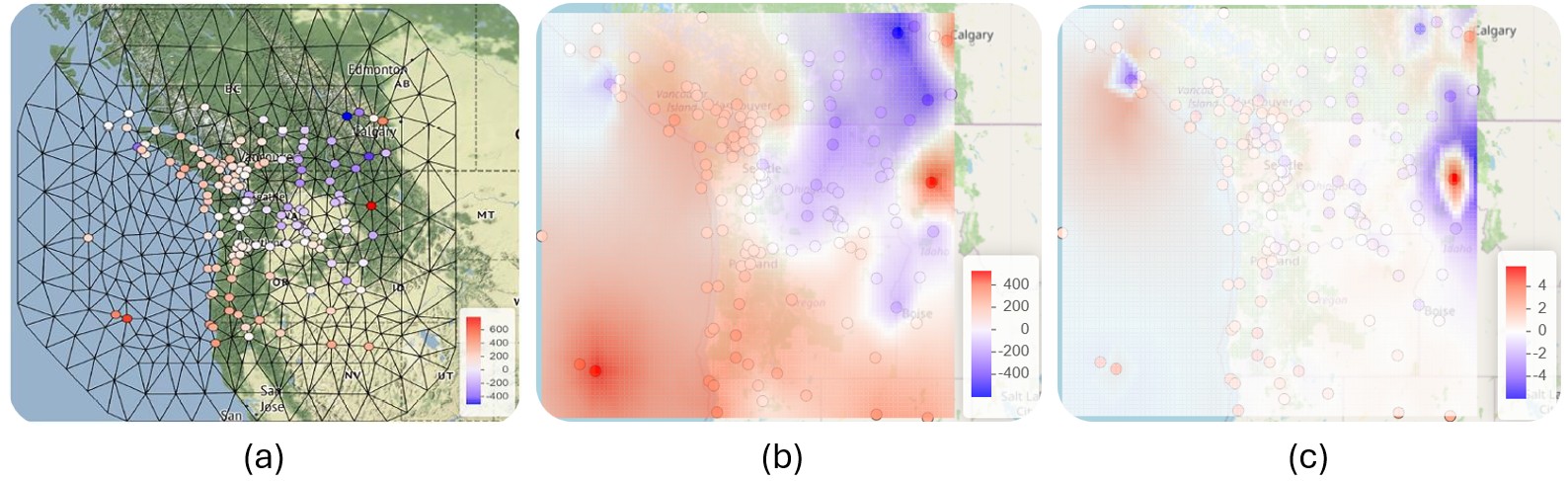 Pressure measurements (a), the LGM's spatial predictions (b), and the
sensitivity of those predictions to relaxing Gaussianity (c). In (c) we see that the Gaussian assumptions oversmooths some local spikes
(red indicates regions where the LnGM model predicts higher pressure).
Usage
LGM <- inla(y ~ f(s, model = "rw1"), data = d, control.compute = list(config = TRUE))

ng.check(LGM)       # is the latent Gaussian assumption adequate? which posterior summaries are most sensitive?
LnGM <- ngvb(LGM)   # fit the non-Gaussian extension

samples <- ngvb_sample(LnGM, n.samples = 30) # sample non-gaussian V from the variational posterior + fit R-INLA models
bayes.factor(samples)               # how much better the LnGM is, with V integrated out?
summary(samples)                    # summary of random effects + fixed effects + hyperparameters of the LnGM
Installation
ngvb builds on INLA, which is not on CRAN, so install it first:
install.packages("INLA",
  repos = c(getOption("repos"), INLA = "https://inla.r-inla-download.org/R/stable"),
  dep = TRUE)

# install.packages("remotes")
remotes::install_github("rafaelcabral-ai/ngvb")
The idea
Every latent Gaussian field is built from a model-specific dependency matrix D that turns
the field x into independent Gaussian increments, D x =ᵈ Λ with Λᵢ ~ N(0, hᵢ) for a known
weight vector h. Its precision is therefore
Q = Dᵀ diag(1/h) D
(D is the difference operator for a random walk, I − ρW for a SAR, κ²C + G for a
Matérn/SPDE, and so on; h is a vector of ones for a random walk and the mesh mass for an
SPDE.) The non-Gaussian extension keeps D and replaces the Gaussian driving noise, giving
each increment its own variance Vᵢ with E[Vᵢ] = hᵢ, which is equivalent to conditioning on
mixing variables V:
Q(θ, V) = D(θ)ᵀ diag(1/V) D(θ)
Where Vᵢ = hᵢ the model is Gaussian; where Vᵢ is inflated the increment is allowed to be
unusually large. A single non-Gaussianity parameter η ≥ 0 controls how far V may stray, and
its exponential prior shrinks back to the Gaussian model unless the data pull away. ngvb fits
this with a variational-Bayes loop that alternates an INLA fit (for fixed V) with closed-form
updates of V and η.
Models
ngvb(fit) and ng.check(fit) auto-detect the component type from the fitted object and
rebuild the operator. No arguments are needed for the auto-detected models:
| Model | f(..., model = ) |
How |
|---|---|---|
| i.i.d. random effects | "iid" |
auto |
| Random walks | "rw1", "rw2" |
auto |
| Autoregressive order 1 | "ar1" |
auto |
| Intrinsic CAR (areal) | "besag" |
auto (graph recovered) |
| Matérn / SPDE | inla.spde2.pcmatern(mesh, prior.range =, prior.sigma =) |
auto (read from the fit) |
| Seasonal | "seasonal" |
auto |
| SAR, proper CAR, OU | — | ngvb_operator() / ngvb_custom() |
| Your own precision, or borrowed from ngme2 | — | ngvb_custom(D, h, ...) |
Additive models just work: each f() term gets its own mixing variables and non-Gaussianity
parameter, all fit jointly.
Documentation
Start with Get started, which covers the model and walks through a time series with jumps. Then pick the article that matches your data:
- Geostatistical data (SPDE)
- Areal data (besag)
- Random intercepts and slopes
- Custom models and ngme2 operators
The reference has the full API.
References
- Cabral, Bolin & Rue (2024). Fitting latent non-Gaussian models using variational Bayes and
Laplace approximations. JASA 119(548):2983–2995.
(the
ngvbmethod) - Cabral, Bolin & Rue (2025). Robustness, model checking, and hierarchical models.
JRSS-B 87(3):632–652. (the
ng.checkdiagnostic)