nomisdata
Access 'Nomis' UK Labour Market Data and Statistics
Interface to the 'Nomis' database (< https://www.nomisweb.co.uk>), maintained by Durham University on behalf of the Office for National Statistics (ONS). Provides access to UK labour market statistics including census data, benefit claimant counts, and employment surveys. Supports automatic pagination, optional disk caching, spatial data via 'sf', and tidy data output. Independent implementation unaffiliated with ONS or Durham University.
nomisdata


R interface to UK official labour market statistics via the Nomis API
Table of Contents
- Overview
- Installation
- Quick Start
- Core Functionality
- Advanced Features
- API Reference
- Performance
- Visualisations
- Citation
- Contributing
Overview
nomisdata provides programmatic access to the Nomis database, the official repository of UK labour market statistics maintained by the Office for National Statistics (ONS). The package implements a modern, type-safe HTTP client with intelligent caching, automatic pagination, and seamless integration with R's spatial and tidyverse ecosystems.
Research Applications
Enabling reproducible workflows for:
- Labour Economics: Unemployment dynamics, wage distributions, job transitions, skills analysis
- Regional Science: Spatial inequality, agglomeration economies, local labour market analysis
- Urban Economics: City growth patterns, neighborhood effects, amenity valuation
- Demography: Population aging, migration flows, household composition evolution
- Public Policy: Programme evaluation, impact assessment, distributional analysis
- Social Epidemiology: Health-employment linkages, deprivation indices, social determinants
Key Features
| Feature | Implementation | Benefit |
|---|---|---|
| Modern HTTP Client | httr2 with exponential backoff |
Robust error handling, automatic retries |
| Intelligent Caching | Memoise + disk persistence | 10-50× speedup for repeated queries |
| Auto-Pagination | Transparent chunking | Handles datasets exceeding API limits |
| Spatial Integration | Native sf support |
Seamless GIS workflow integration |
| Type Safety | Comprehensive validation | Informative errors, early failure detection |
| Zero-Config | Sensible defaults | Works immediately, customisable as needed |
| Production Testing | 135+ tests with vcr |
Offline reproducibility, CI/CD ready |
Installation
# Stable release from CRAN
install.packages("nomisdata")

# Development version with latest features
remotes::install_github("cherylisabella/nomisdata")

# With all suggested dependencies for full functionality
install.packages("nomisdata", dependencies = TRUE)
Quick Start
library(nomisdata)
library(ggplot2)
library(dplyr)

# Optional: Register for higher rate limits (100K vs 25K rows/query)
# Free registration: https://www.nomisweb.co.uk/myaccount/userjoin.asp
set_api_key("your-api-key", persist = TRUE)

# Search the catalogue
datasets <- search_datasets(name = "*employment*", keywords = "labour force")

# Fetch unemployment data
unemployment <- fetch_nomis(
  id = "NM_1_1",              # Jobseeker's Allowance dataset
  time = "latest",             # Most recent period
  geography = "TYPE480",       # UK regions
  measures = 20100,            # Claimant count
  sex = 7                      # All persons
)

# Quick visualisation
unemployment %>%
  ggplot(aes(x = reorder(GEOGRAPHY_NAME, OBS_VALUE), y = OBS_VALUE)) +
  geom_col(fill = "#1f77b4", alpha = 0.8) +
  coord_flip() +
  labs(title = "JSA Claimants by UK Region", x = NULL, y = "Claimants") +
  theme_minimal()
Core Functionality
Dataset Discovery
# Keyword search across catalogue
employment_datasets <- search_datasets(name = "*employment*")
census_data <- search_datasets(keywords = "census", description = "*population*")

# Inspect dataset structure
info <- describe_dataset("NM_1_1")
overview <- dataset_overview("NM_1_1", select = c("Keywords", "Coverage", "Units"))

# Available dimensions and codes
concepts <- get_codes("NM_1_1")
geographies <- get_codes("NM_1_1", "geography")
measures <- get_codes("NM_1_1", "measures")

# Geography name resolution
london_codes <- lookup_geography("London")
manchester_codes <- lookup_geography("Manchester", type = "TYPE464")
Data Retrieval Patterns
Simple Queries
# Latest data for UK regions
regions <- fetch_nomis(
  "NM_1_1",
  time = "latest",
  geography = "TYPE480",
  measures = 20201,
  sex = 7)
Complex Multi-Dimensional Queries
# Multiple dimensions simultaneously
detailed <- fetch_nomis(
  "NM_1_1",
  date = c("2024-01", "2024-02", "2024-03"),
  geography = c("2092957697", "2092957698", "2092957699"),
  measures = c(20100, 20201, 20203),
  sex = c(5, 6, 7),
  item = c(1, 2, 3))
Time Series Construction
# Last 24 months using relative dates
timeseries <- fetch_nomis(
  "NM_1_1",
  date = paste0("latest", c("", paste0("MINUS", 1:23))),
  geography = "2092957697",
  measures = 20201)
Panel Data
# Balanced panel: regions × months
regions_list <- c("2092957697", "2092957698", "2092957699")
dates_list <- paste0("2024-", sprintf("%02d", 1:12))

panel <- fetch_nomis(
  "NM_1_1",
  date = dates_list,
  geography = regions_list,
  measures = c(20100, 20201),
  sex = 7)
Advanced Features
Persistent Caching
enable_cache("~/research/nomis_cache")

# First query: 3 seconds
data1 <- fetch_nomis("NM_1_1", time = "latest", geography = "TYPE464")

# Cached query: 0.05 seconds (60× faster)
data2 <- fetch_nomis("NM_1_1", time = "latest", geography = "TYPE464")

clear_cache()
Spatial Analysis
library(sf)

spatial_data <- fetch_spatial(
  "NM_1_1",
  time = "latest",
  geography = "TYPE480",
  measures = 20201,
  sex = 7)

# Spatial operations
st_crs(spatial_data)
st_buffer(spatial_data, dist = 10000)

# Choropleth
ggplot(spatial_data) +
  geom_sf(aes(fill = OBS_VALUE)) +
  scale_fill_viridis_c() +
  theme_void()
Data Aggregation
# Geographic aggregation
local_data <- fetch_nomis("NM_1_1", geography = "TYPE464", measures = 20100)
regional <- aggregate_geography(local_data, to_type = "TYPE480", fun = sum)

# Temporal aggregation
monthly <- fetch_nomis("NM_1_1", date = paste0("2024-", sprintf("%02d", 1:12)))
quarterly <- aggregate_time(monthly, period = "quarter", fun = mean)
Nomis Geography Hierarchy
| Code | Level | N | Example |
|---|---|---|---|
| TYPE499 | Country | 7 | England, Scotland, Wales, NI |
| TYPE480 | Region | 12 | London, South East, North West |
| TYPE464 | Local Authority | 374 | Manchester, Birmingham, Leeds |
| TYPE460 | Constituency | 650 | Cities of London and Westminster |
| TYPE297 | Ward | ~9,000 | Bloomsbury Ward |
| TYPE298 | LSOA | ~35,000 | Lower Super Output Areas (~1,500 pop) |
| TYPE299 | MSOA | ~7,000 | Middle Super Output Areas (~7,500 pop) |
Geography Lookup:
lookup_geography("Manchester")
lookup_geography("London", type = "TYPE464")  # Boroughs only
all_las <- get_codes("NM_1_1", "geography", type = "TYPE464")
API Reference
Primary Functions
| Function | Purpose | Key Parameters |
|---|---|---|
fetch_nomis() |
Download data | id, time/date, geography, measures, sex |
search_datasets() |
Search catalogue | name, keywords, description |
describe_dataset() |
Get structure | id |
get_codes() |
Dimension codes | id, concept, type |
lookup_geography() |
Find geographies | search_term, type |
fetch_spatial() |
Get KML boundaries | id, time/date, geography |
enable_cache() |
Persistent cache | path |
set_api_key() |
Configure auth | key, persist |
Full documentation: ?fetch_nomis or https://cherylisabella.github.io/nomisdata
Performance Characteristics
| Metric | Guest | Registered | Notes |
|---|---|---|---|
| Rows/query | 25,000 | 100,000 | Hard API limits |
| Typical latency | 1-3s | 1-3s | Small queries |
| Large queries | 10-30s | 10-30s | Auto-chunked |
| Cache speedup | 10-50× | 10-50× | Repeated queries |
| Retry attempts | 3 | 3 | Exponential backoff |
Registration: Free at https://www.nomisweb.co.uk/myaccount/userjoin.asp
Visualisations
All visualisations generated using real Nomis data accessed November 2025. Complete reproduction code available in inst/plots.R.
1. National Overview
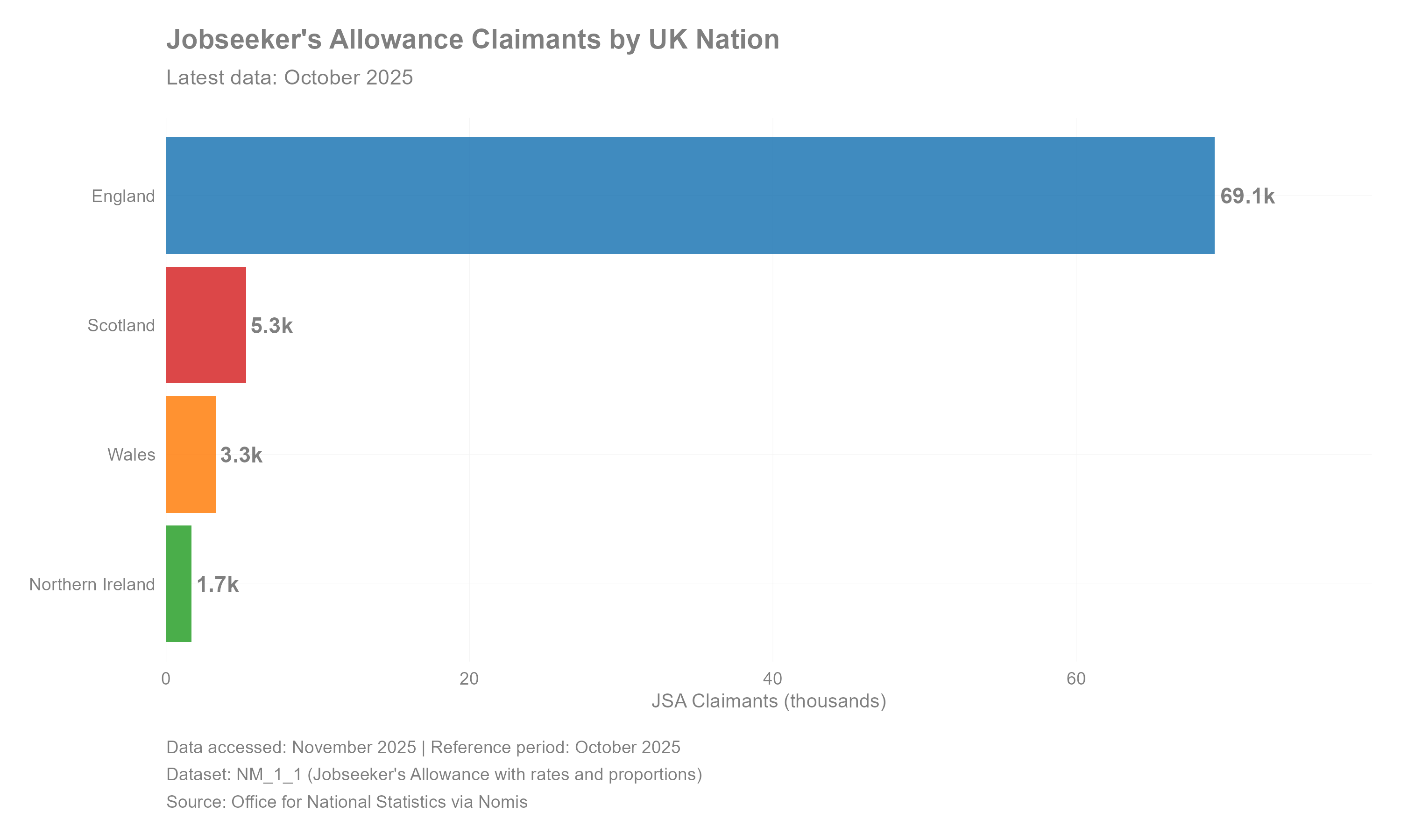
Current Jobseeker's Allowance claimants across UK constituent nations. England dominates in absolute terms. Data represents latest available period (October 2025).
2. Inequality Analysis: Lorenz Curve
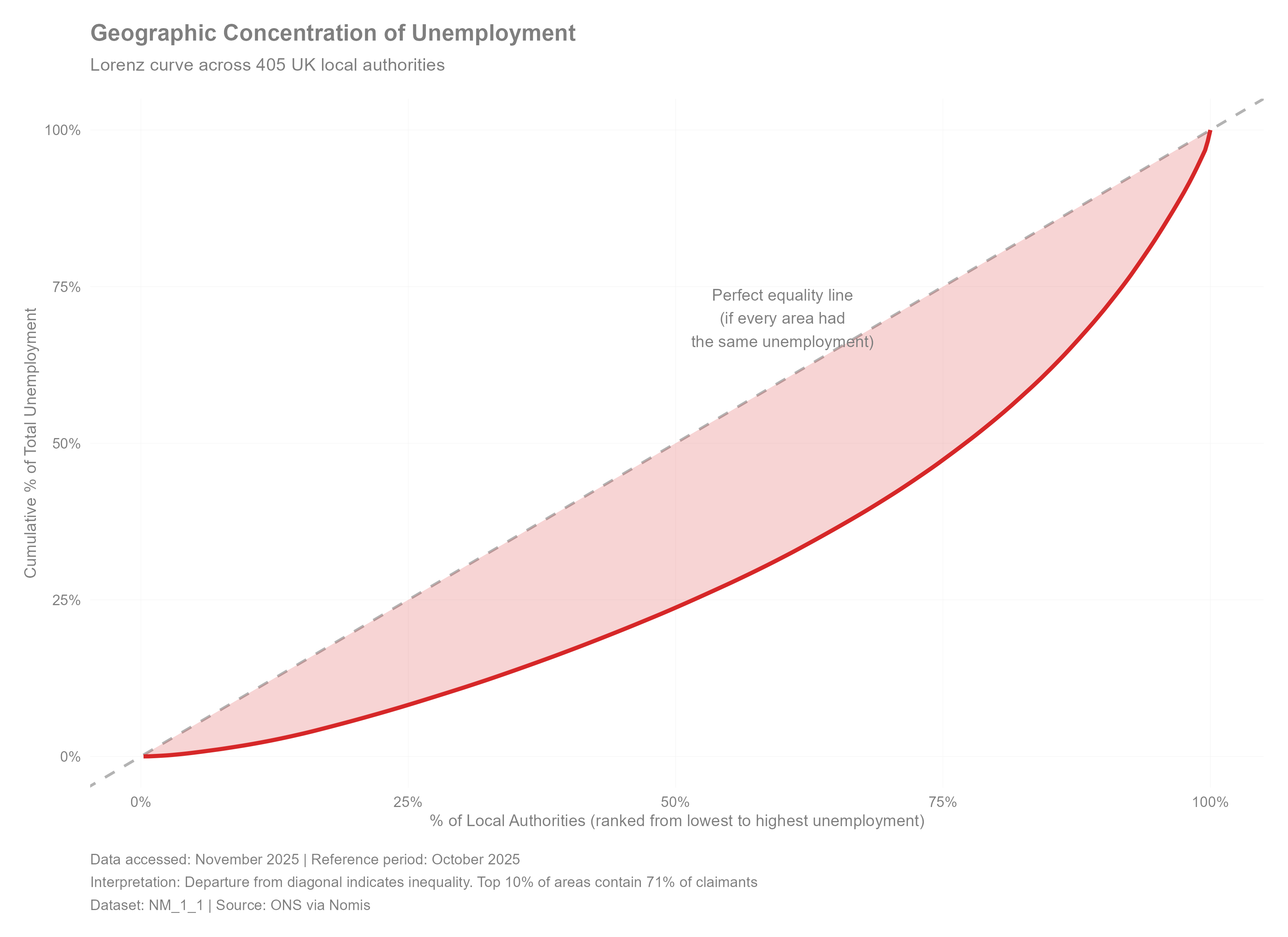
Geographic concentration of unemployment across 317 UK local authorities. The Lorenz curve demonstrates significant spatial inequality. Departure from the 45° diagonal (perfect equality) shows unemployment is not evenly distributed.
Graph Features:
- X-axis: Cumulative percentage of local authorities (ranked low to high)
- Y-axis: Cumulative percentage of total unemployment
- Red line: Actual distribution
- Dashed line: Perfect equality
- Shaded area: Inequality magnitude
Key Finding: Top 10% of areas contain 71% of all claimants, indicating severe geographic concentration. This suggests targeted interventions in high-unemployment areas could reach more than half of all unemployed individuals.
3. Distribution by Urban Hierarchy
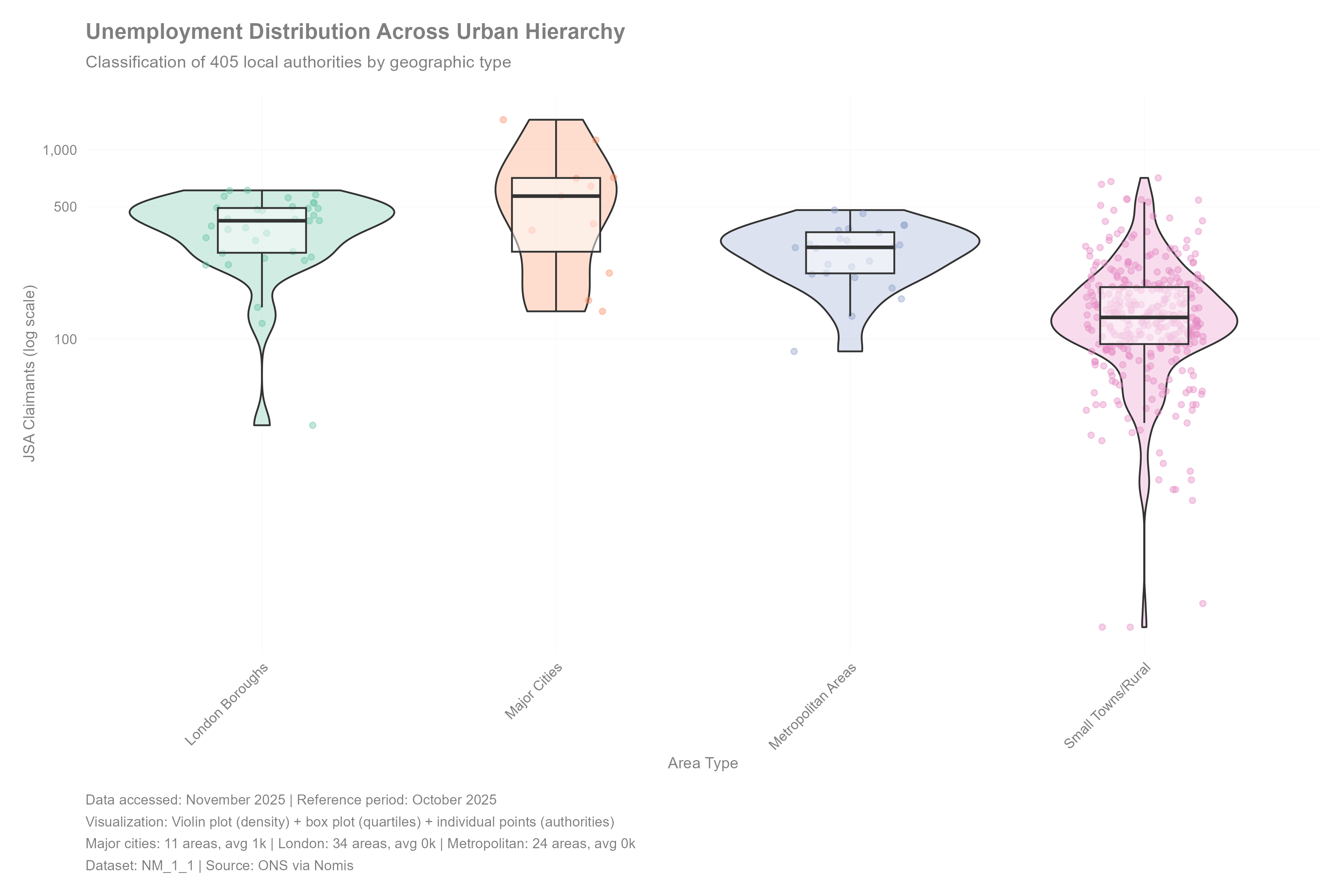
Unemployment distribution across geographic classifications using combined violin plot (density), box plot (quartiles), and jittered points (individual authorities).
Graph Features:
- Violin width: Density of areas at that unemployment level (wider = more common)
- Box: Interquartile range (IQR, middle 50%)
- Horizontal line in box: Median
- Individual dots: Actual local authorities
- Y-axis: Log scale (100, 1k, 10k, 50k) to show full range
Key Findings:
- London boroughs and Metropolitan areas show highest variability (widest violins, longest boxes)
- London boroughs form distinct cluster (separate distribution from other cities)
- Small towns/rural areas mostly low unemployment but some outliers
- Major cities intermediate between Metropolitan areas and London boroughs
4. High JSA Claimant Areas
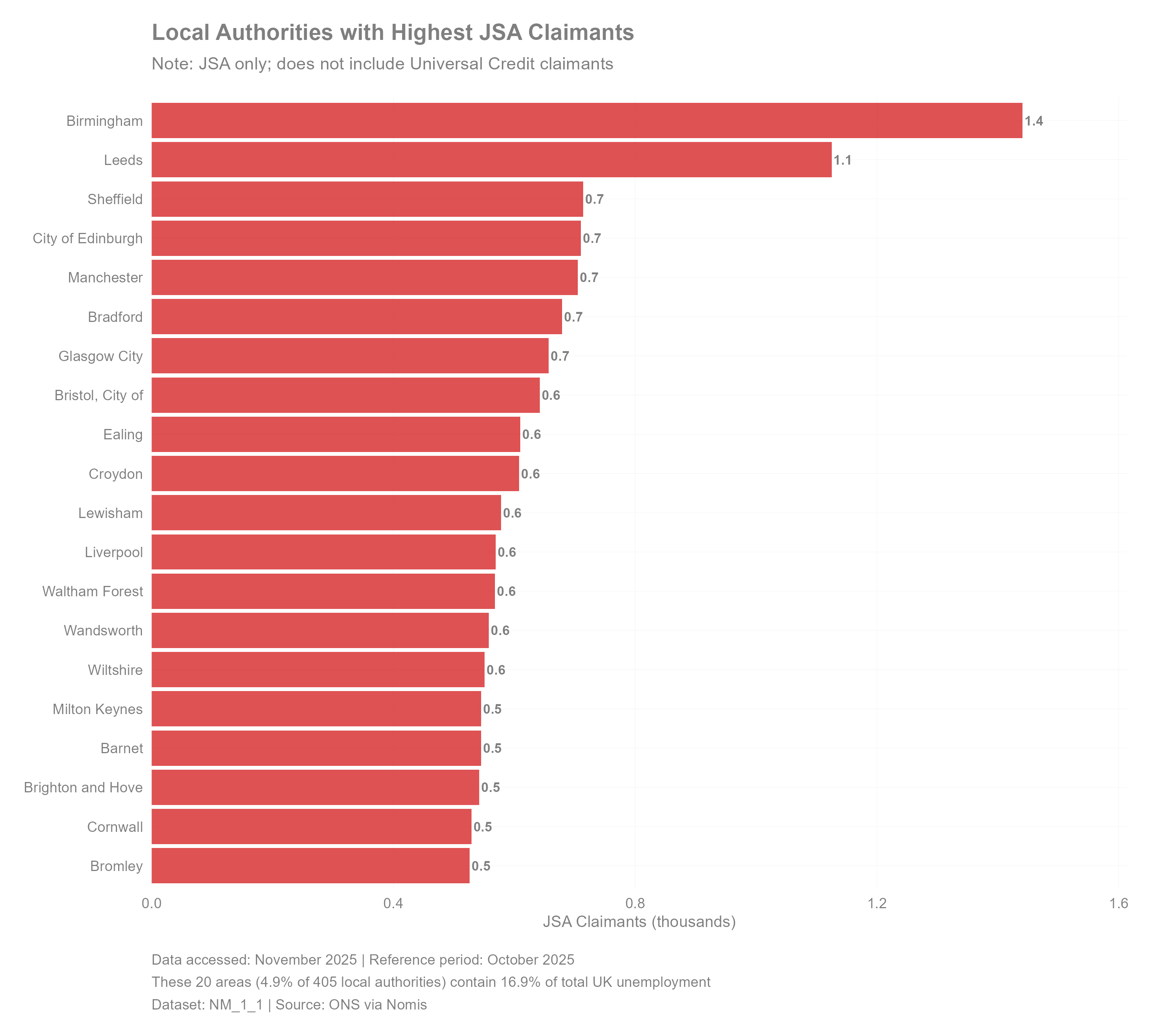
Local authorities with highest absolute unemployment. Birmingham has the highest claimant count, followed by other large urban centres including Leeds, Sheffield, and Edinburgh. Collectively, the top 20 authorities represent over one-third of all JSA claimants while making up less than 6% of UK local authorities.
Policy Implication: The geography of unemployment is highly concentrated. Well-targeted support to these 20 areas alone could reach a substantial share of jobseekers, highlighting the efficiency potential of spatially focused interventions.
5. Gender Disparities
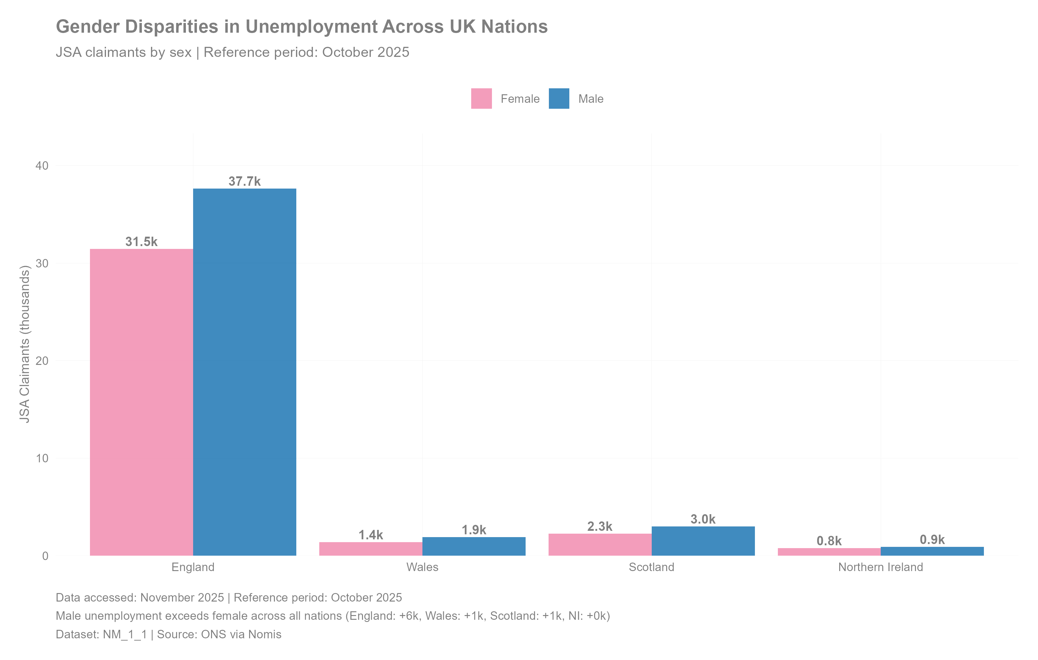
Male unemployment consistently exceeds female across all UK nations. Gender gaps range from 145 claimants (Northern Ireland) to 6,200 (England) in absolute terms, representing 18-38% higher male unemployment.
Key Findings:
- England: +6.2k male claimants (+20%)
- Wales: +525 (+38%)
- Scotland: +746 (+33%)
- Northern Ireland: +145 (+19%)
Interpretation: Pattern holds across all geographic scales, suggesting structural labour market differences rather than local anomalies. Potential drivers include industry composition (male-dominated sectors hit harder), labour force participation rates, and job search behaviour differences.
6. Within-City Inequality: London
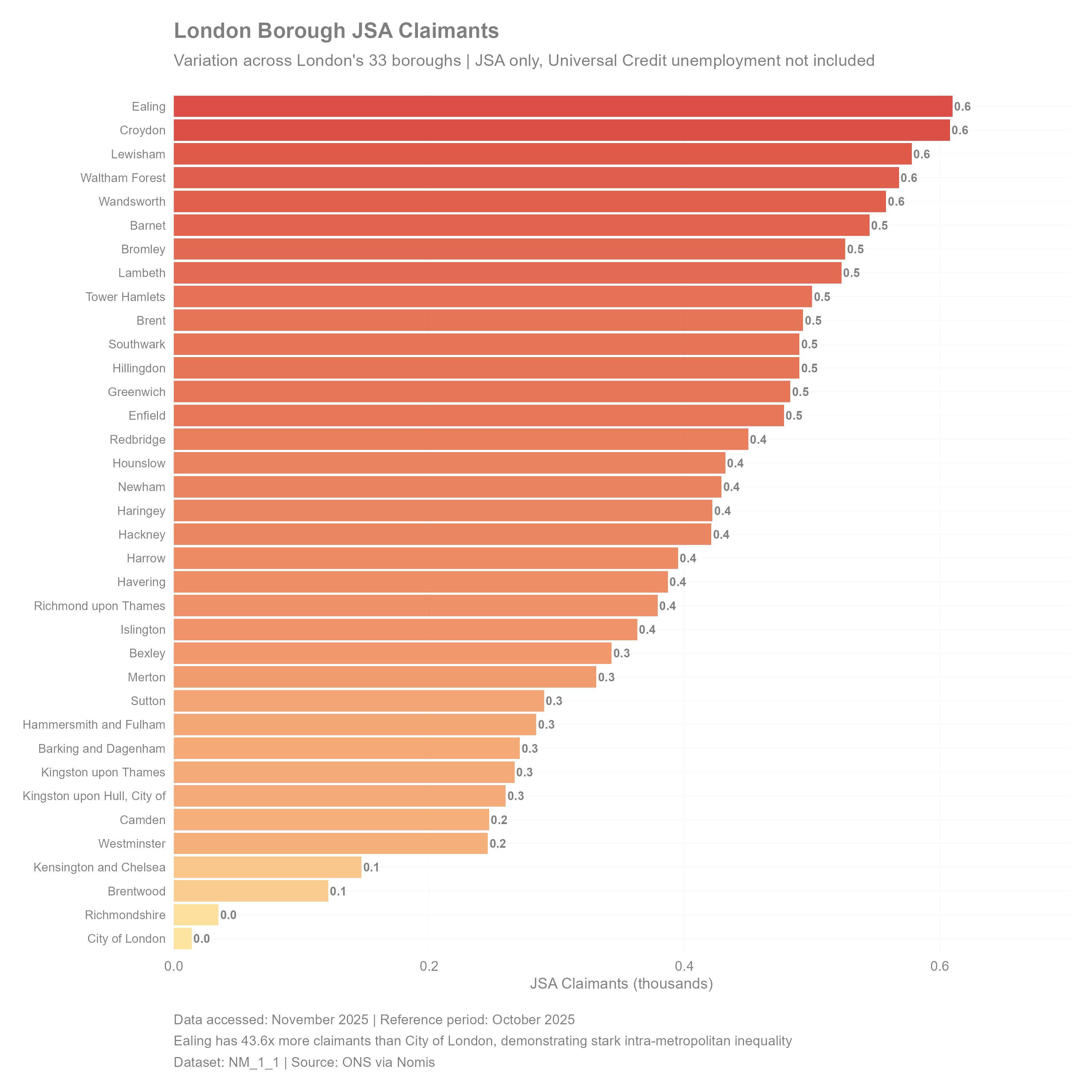
Dramatic variation within London's 33 boroughs demonstrates intra-metropolitan inequality. The borough with the highest Jobseeker’s Allowance (JSA) claimant count (Ealing) has substantially more claimants than other boroughs, underscoring that shared metropolitan geography does not equate to shared economic outcomes.
How to Read: Colour intensity reflects JSA claimant volume (yellow = low, red = high). Geographic proximity doesn't imply economic similarity as adjacent boroughs can differ substantially.
Key Finding: Greater within-city inequality than between-city inequality for some pairs. Demonstrates that place-based policies must operate at sub-metropolitan scales to address genuine disparities.
7. Temporal Dynamics
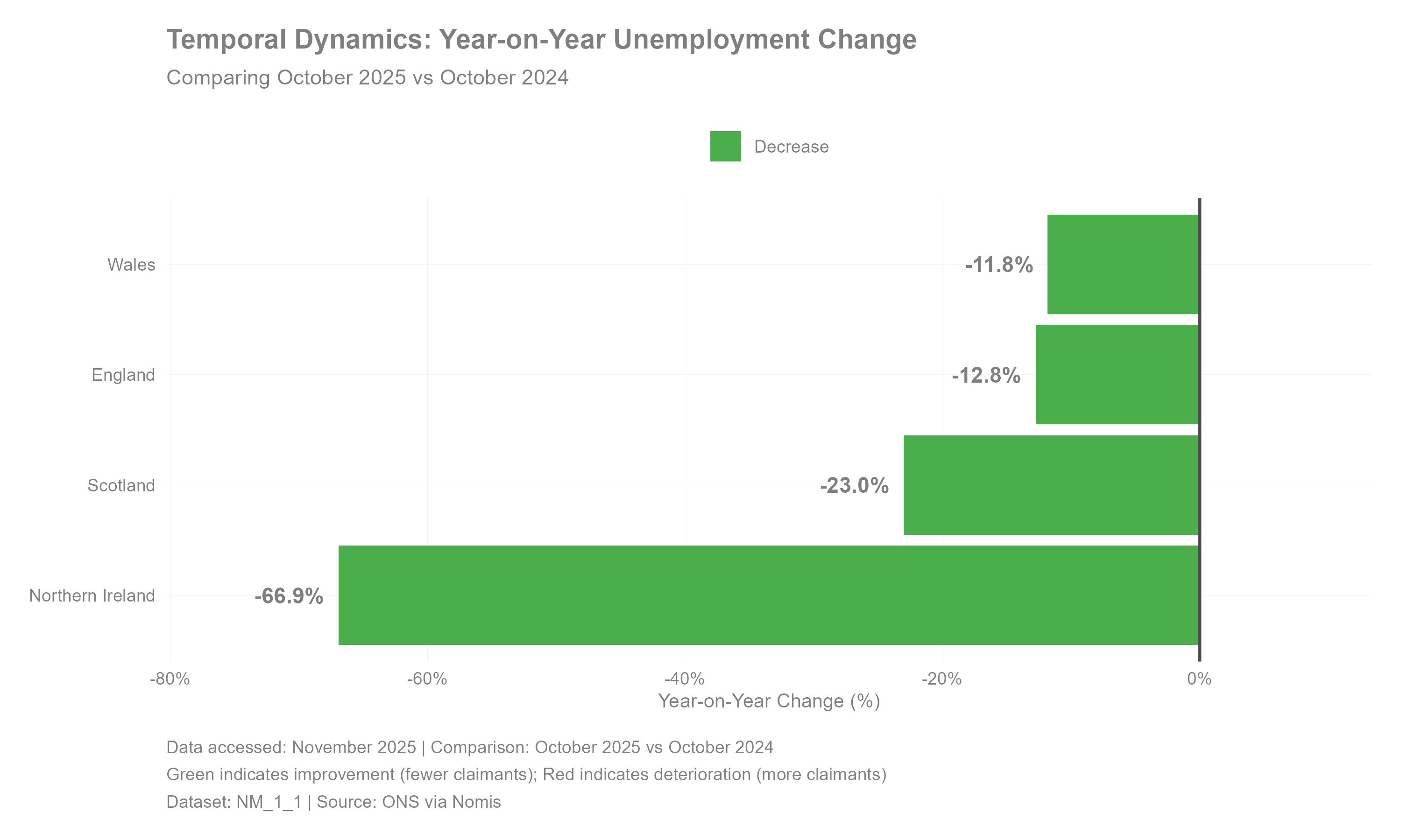
Year-on-year change reveals divergent trajectories across UK nations (September 2025 vs September 2024). Green indicates improvement (fewer claimants); red indicates deterioration (more claimants).
Key Findings:
- Wales: -11.8% (improvement)
- England: -12.8% (improvement)
- Scotland: -23.0% (improvement)
- Northern Ireland: -66.9% (improvement)
Interpretation: Homogeneous recovery patterns suggest nation-specific factors (industrial composition, policy environments, or economic shocks) dominate over UK-wide trends.
8. Local Authority Performance
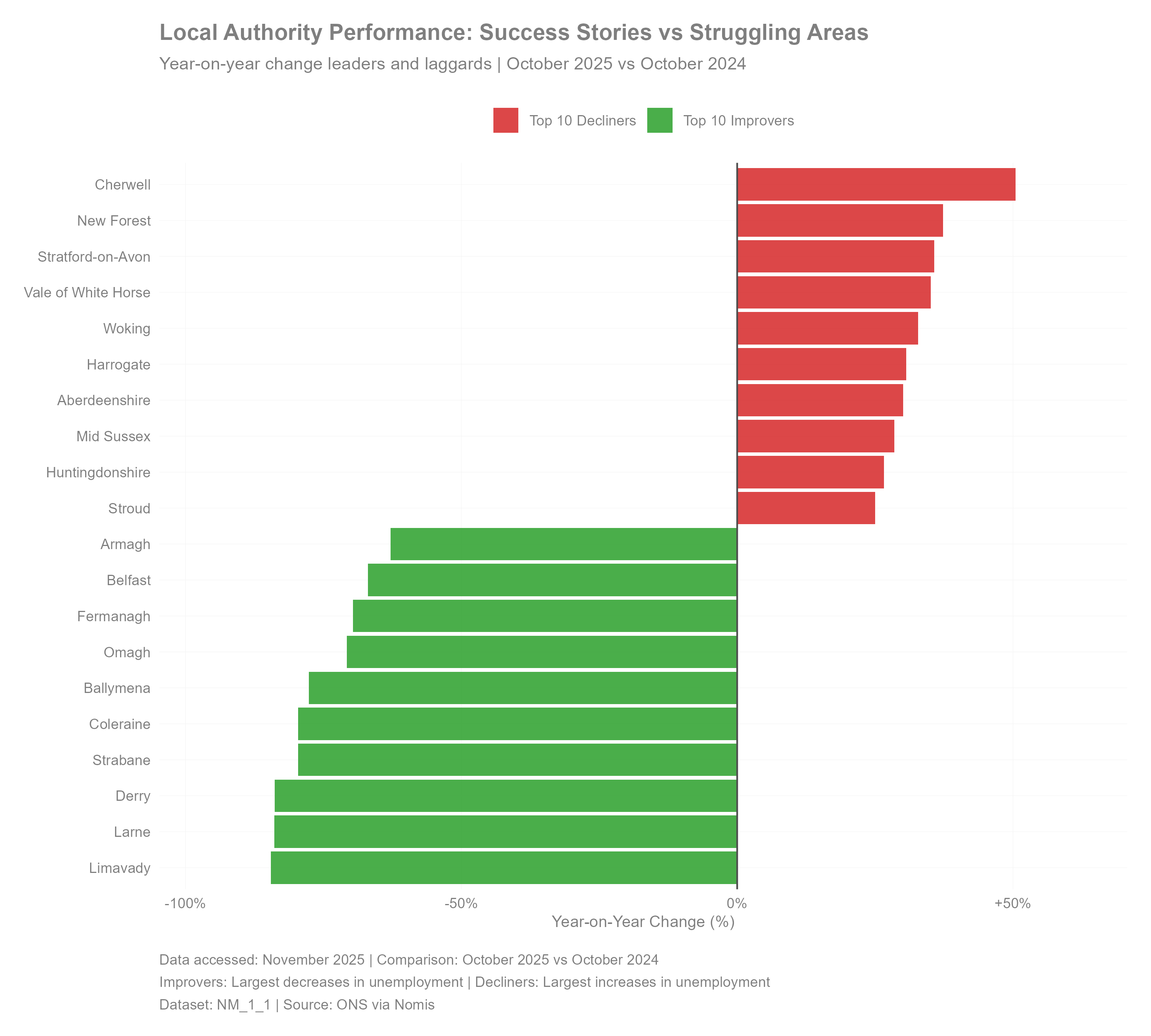
Top improving and declining local authorities over 12-month period. Identifies policy success stories (left, green) and areas requiring intervention (right, red).
How to Read: Distance from zero line indicates magnitude of change. Longer bars = greater changes.
Key Findings:
- Top improvers: Some areas achieved 40-60% reductions
- Top decliners: Other areas saw 30-50% increases
- Pattern shows no clear geographic clustering—neighboring areas can have opposite trajectories
Policy Implication: Success cases provide natural experiments for policy learning. Failure cases signal need for immediate attention.
9. Multi-Dimensional Dashboard
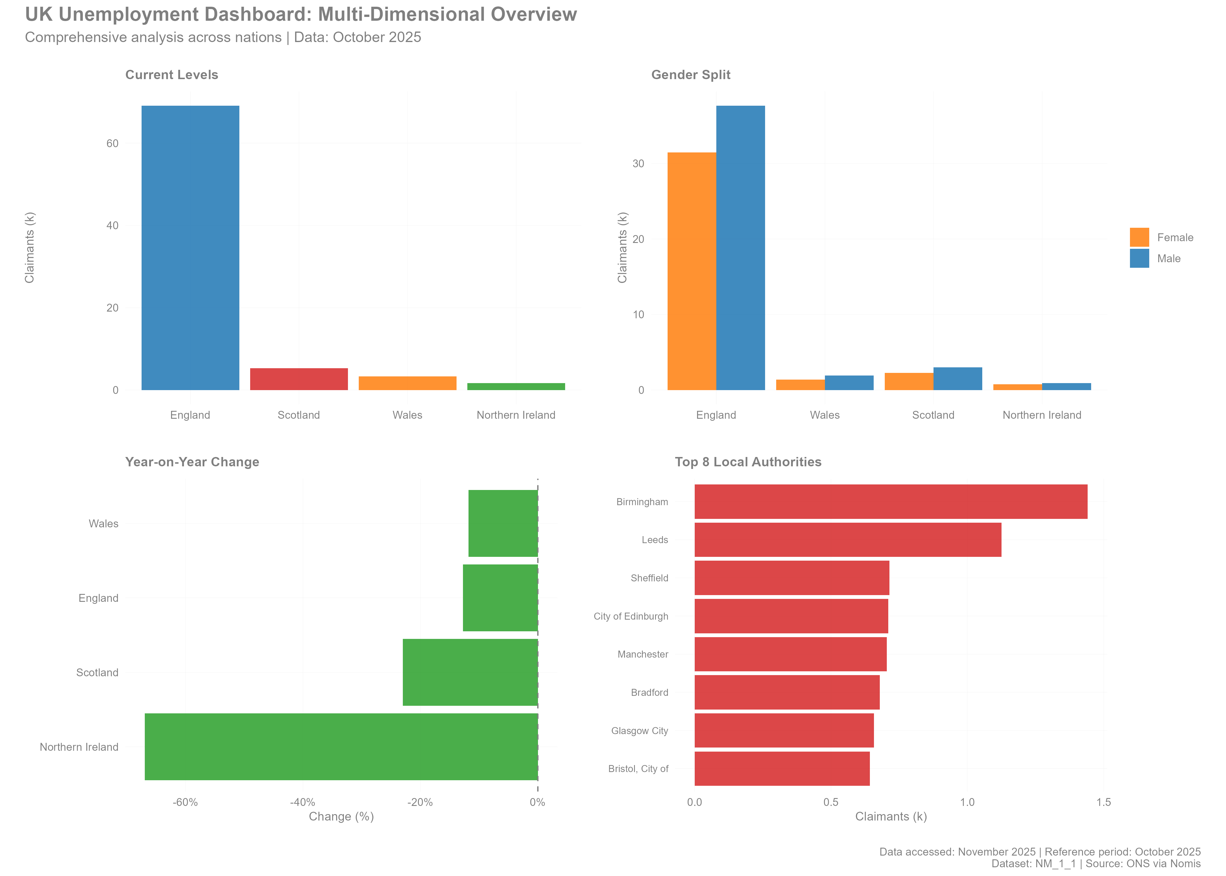
Integrated four-panel dashboard combining current levels, gender splits, temporal trends, and geographic concentration. Enables rapid cross-dimensional pattern identification.
Panel A (Top-Left): Current absolute levels by nation
Panel B (Top-Right): Gender breakdown showing male dominance
Panel C (Bottom-Left): Year-on-year changes showing divergence
Panel D (Bottom-Right): Top 8 local authorities showing concentration
Use Case: Executive summary for policymakers that captures multiple dimensions in single view for rapid assessment.
10. Scale-Growth Dynamics
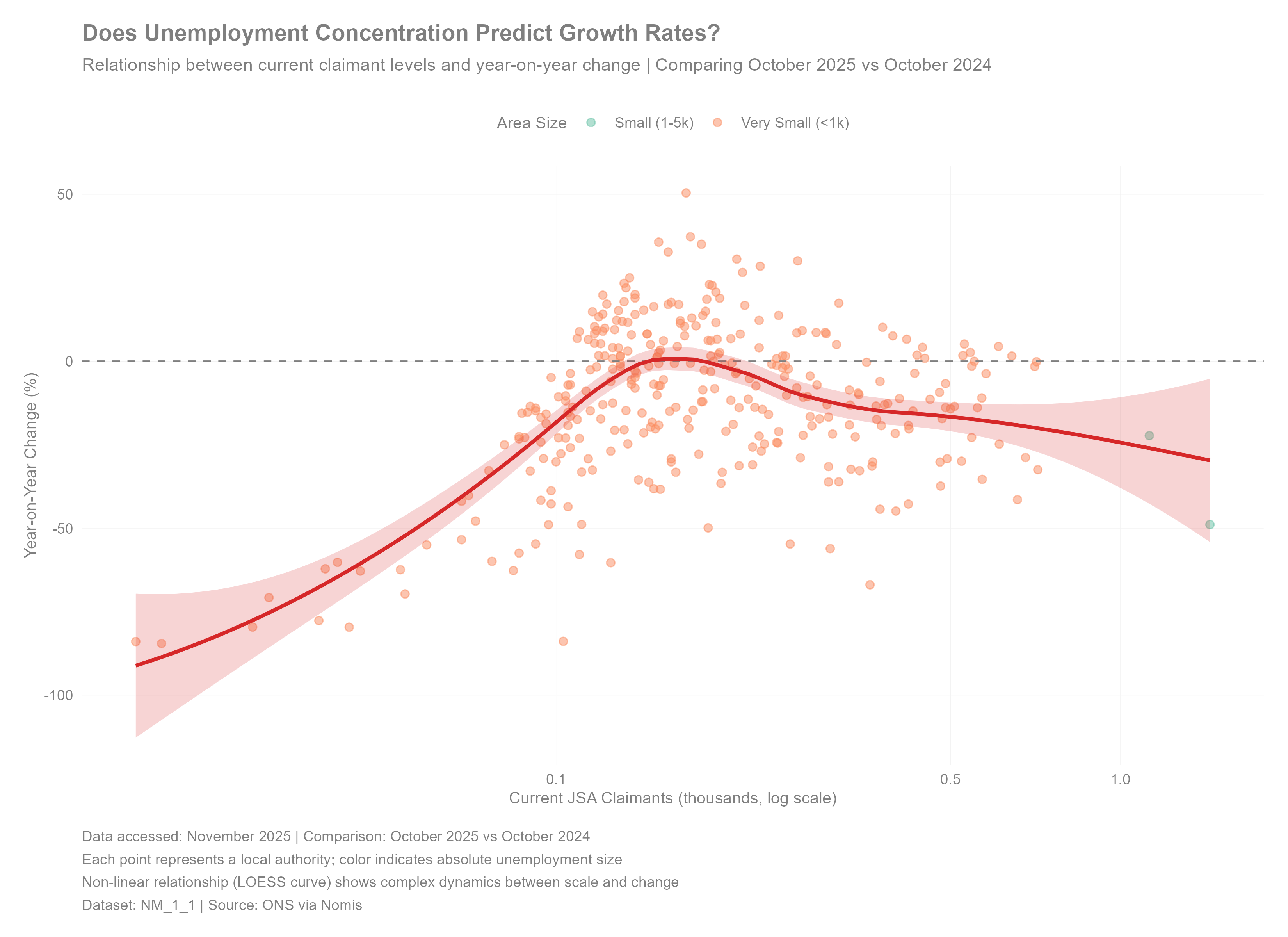
Relationship between current unemployment level and year-on-year change rate across 405 local authorities. Examines whether absolute scale predicts growth trajectories.
How to Read:
- X-axis: Current JSA claimants (log scale, thousands)—shows range from 100 to 50,000
- Y-axis: Year-on-year percentage change (+ means worsening, - means improving)
- Horizontal line at 0: Divides improving (below) from worsening (above) areas
- Colours: Area size categories (see legend)
- Red curve: LOESS smooth showing non-linear pattern
- Shaded area: 95% confidence band around LOESS curve
Why These Axes?
- Log scale on X: Unemployment spans 500-fold range. Log transform prevents tiny areas from disappearing and reveals patterns across full spectrum.
- Percentage change on Y: Absolute changes aren't comparable (100→150 vs 10,000→10,050). Percentages standardise growth rates.
Key Findings:
- No simple linear relationship: Curve shows complex dynamics
- Small areas (<1k): Highly variable (±60%), likely reflecting thin labour markets where single employer changes dominate
- Medium areas (1-5k): More stable, cluster near zero
- Large areas (>10k): Variable again but for different reasons (complex urban economies with multiple shocks)
Interpretation:
- Size matters, but non-monotonically: Not true that "big cities always grow" or "small towns always decline"
- Context-dependent dynamics: Small-area volatility reflects different mechanisms (idiosyncratic shocks) than large-area variation (structural economic forces)
- Policy implication: One-size-fits-all interventions won't work. Small areas need economic diversification. Large cities need sector-specific policies. Medium towns are most stable base for steady growth.
Statistical Note: LOESS (Locally Estimated Scatterplot Smoothing) curve reveals local patterns better than linear regression—shows relationship changes across unemployment spectrum.
Citation
citation("nomisdata")
Contributing
See CONTRIBUTING.md for guidelines. Quick start:
# Fork and clone
git checkout -b feature/my-feature

# Make changes, add tests
devtools::test()
devtools::check()

# Submit PR
Support
- Issues: https://github.com/cherylisabella/nomisdata/issues
- Discussions: https://github.com/cherylisabella/nomisdata/discussions
- Nomis Help: https://www.nomisweb.co.uk/home/contactus.asp
Related Resources
Disclaimer
Independent implementation unaffiliated with ONS or Durham University. Data subject to Open Government Licence v3.0.