Sensitivity Analysis of Omitted Variable Bias

Conduct sensitivity analysis of omitted variable bias in linear econometric models using the methodology presented in Basu (2025) .

ovbsa

The goal of ovbsa (omitted variable bias sensitivity analysis) is to conduct sensitivity analysis of reported results in linear econometrics models to the presence of omitted variable bias. The key function in this package computes a bias-adjusted confidence interval by implementing the method presented in Basu (2026), which, in turn, builds on and extends Cinelli and Hazlett (2020).

Consider the linear regression of an outcome, $Y$ , on a treatment, $D$, a set of observed covariates, $X$, and an unobserved confounder, $Z$. Choose a regressor, $X_j$, that is included in the model, as a benchmark covariate. Let $k_D$ and $k_Y$ denote sensitivity parameters.

Here $k_D$ captures the strength of association of $Z$ with $D$ relative to the strength of association of the benchmark covariate, $X_j$, with $D$. Similarly, $k_Y$ captures the strength of association of $Z$ with $Y$ relative to the strength of association of $X_j$ with $Y$. The strengths of associations are measured with partial R-squared conditional on all the regressors other than the benchmark covariate, $X_j$.

Cinelli and Hazlett (2020) had presented a method to compute omitted variable bias-adjusted confidence intervals for specific values of $k_D$ and $k_Y$. Basu (2026) asks us to consider $k_D$ and $k_Y$ as random variables, identifies their supports, imposes reasonable prior distributions on these random variables and then computes bias-adjusted confidence intervals by integrating out $k_D$ and $k_Y$ over their supports.

In this package, I use independent truncated exponential distributions as prior distribution of $k_D$ and $k_Y$. For more details see Basu (2026).

Installation

You can install the package ovbsa from CRAN with:

# uncomment this line
# install.packages("ovbsa")

You can install the development version of ovbsa from GitHub with:

# uncomment these lines
# install.packages("pak")
# pak::pak("dbasu-umass/ovbsa")

Main function

The main function in this package is:

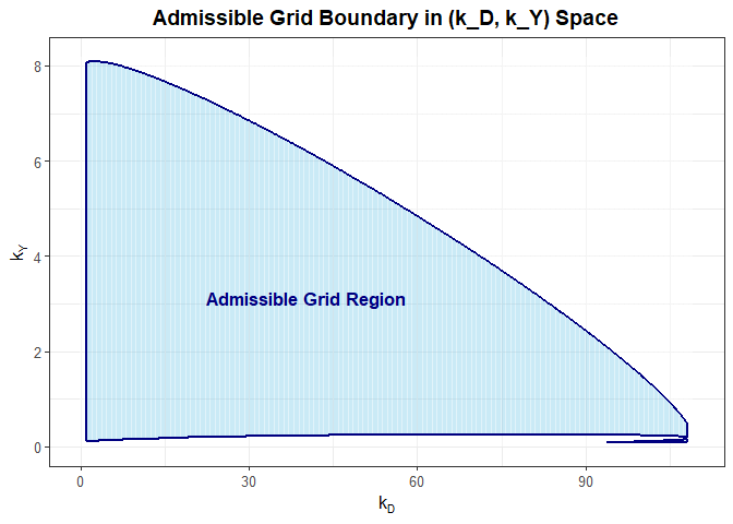
baci: this function computes the Bias-Adjusted Confidence Interval (baci) in a linear regression model when $k_D$ and $k_Y$ follow truncated exponential distributions; the function returns a list results containing the unadjusted and bias-adjusted confidence intervals; it also returns a list undstats containing the estimate, the unadjusted stamdard error, the max of $k_D$ and the max of $k_Y$; it also returns a ggplot2 plot object visualizing the support of the joint distribution of $(k_D,k_Y)$.

Let us first load the relevant libraries and then work through an example.

library(ovbsa)
library(sensemakr)
#> See details in:
#> Carlos Cinelli and Chad Hazlett (2020). Making Sense of Sensitivity: Extending Omitted Variable Bias. Journal of the Royal Statistical Society, Series B (Statistical Methodology).
library(ggplot2)

In the examples we will use use the data set darfur from the package sensemakr, which studies the effect of exposure to violence ($D$) on attitudes towards peace ($Y$) holding a set of covaraites constant ($X$). The researchers suspects there is an omitted variable ($Z$) and uses female as the benchmark covariate, $X_j$.

Bias-adjusted confidence interval

This is a basic example which shows you how to find the bias-adjusted estimate, the bias-adjusted standard error and the bias-adjusted confidence interval in a linear regression model.

To use this function the user needs to choose a benchmark covariate (which we have already done), the significance level alpha for testing the null hypothesis that the treatment effect is zero, N to create a grid of size $N \times N$ over the support of the distribution of $(k_D,k_Y)$ and the medians of the distributions of $k_D$ and $k_Y$ respectively.

The default values of these medians are each set to $1$ (to capture the idea that the unobserved confounder is as likely to be more strongly associated with the outcome/treatment as less). If this default seems reasonable, then the user does not need to choose the medians. Otherwise, she can choose specific values for medkd (median of the distribution of $k_D$) and medky (median of the distribution of $k_D$).

Here we choose the benchmark covariate as female, alpha=0.05 and N=1000 (we use the default values for the medians of the distributions of $k_D$ and $k_Y$).

In the first step of the analysis, we estimate the model with ordinary least squares using the lm function.

## fit model
fit <- lm(peacefactor ~ directlyharmed + age + farmer_dar + herder_dar +
             pastvoted + hhsize_darfur + female + village,
             data = sensemakr::darfur)

In the second step, we call baci to conduct sensitivity analysis.

# conduct sensitivity analysis
res1 <- ovbsa::baci(fit = fit, treatment = "directlyharmed",
                benchmark = "female", N = 1000, alpha = 5/100)
#> Extracting regression quantities : 0.83 sec elapsed
#> Computing values on the grid : 0.36 sec elapsed
#> Prior distribution: truncated exponential : 1.16 sec elapsed
#> Results available now!

Let us see the results, starting with the underlying statistics:

res1$undstats
#>                 Values
#> estimate    0.09731582
#> std error   0.02325654
#> max(kD)   109.11924031
#> max(kY)     8.17145822

The unadjusted estimate and standard errors are 0.097 and 0.023 respectively. We also see that the maximum values that $k_D$ and $k_Y$ can take are 109.12 and 8.17, respectively. Thus, the support of $k_D$ is [0, 109.12] and the support of $k_Y$ is [0,8.17].

Let us now see the unadjusted and bias-adjusted confidence intervals.

res1$results
#>                       Lower     Upper
#> Unadjusted CI    0.05166327 0.1429684
#> Bias-adjusted CI 0.02596471 0.1234509

The unadjusted 95% confidence interval is [0.052,0.142] and the bias-adjusted 95% confidence interval is [0.026,0.123]. Thus, even after taking account of possible omitted variable bias, the reported results holds: exposure to violence has a positive impact on the attitude towards peace; the effect does not wash out once we take account of omitted variable bias.

Finally, let us see a picture of the support of the joint prior distribution of $k_D$ and $k_Y$.

print(res1$support_kdky_plot)

While above we have computed the 95% bias-adjusted confidence interval, we can change the significane level easily. Here, let us compute the 90% and 99% bias-adjusted confidence intervals.

# conduct sensitivity analysis: 90% conf int
res2 <- ovbsa::baci(fit = fit, treatment = "directlyharmed",
                benchmark = "female", N = 1000, alpha = 10/100)
#> Extracting regression quantities : 0.72 sec elapsed
#> Computing values on the grid : 0.18 sec elapsed
#> Prior distribution: truncated exponential : 0.87 sec elapsed
#> Results available now!
# conduct sensitivity analysis: 99% conf int
res3 <- ovbsa::baci(fit = fit, treatment = "directlyharmed",
                benchmark = "female", N = 1000, alpha = 1/100)
#> Extracting regression quantities : 0.72 sec elapsed
#> Computing values on the grid : 0.26 sec elapsed
#> Prior distribution: truncated exponential : 1.07 sec elapsed
#> Results available now!

Now let us see the results.

# 90% conf int
res2$results
#>                       Lower     Upper
#> Unadjusted CI    0.05901691 0.1356147
#> Bias-adjusted CI 0.03388222 0.1157064

# 99% conf int
res3$results
#>                       Lower     Upper
#> Unadjusted CI    0.03726458 0.1573671
#> Bias-adjusted CI 0.01039368 0.1385320

Thus, we have replicated the second row in panel A, Table 1 in Basu (2026).

References

Basu, D. (2026). Approximate omitted variable bias-adjusted confidence intervals Economics Letters. DOI: 10.1016/j.econlet.2026.113248
Cinelli, C. and Hazlett, C. (2020). Making Sense of Sensitivity: Extending Omitted Variable Bias. Journal of the Royal Statistical Society Series B: Statistical Methodology, 82(1):39–67. DOI: 10.1111/rssb.12348