bartisan
Generalized Bayesian Additive Regression Trees
Fits Bayesian additive regression trees (BART) models for
likelihoods outside the conditionally conjugate Gaussian case, using the
Laplace-approximation reversible-jump sampler of Linero (2025)
bartisan: Generalized Bayesian Additive Regression Trees
Overview
Bayesian additive regression trees (BART) estimate a regression function as a sum of small trees, so nonlinearity and interactions are found rather than specified. bartisan does that for response distributions that standard BART cannot reach, using the Laplace-approximation reversible-jump sampler of Linero (2025), which relaxes the requirement that the leaf parameters be integrable in closed form. That requirement ties standard BART to a Gaussian likelihood. Relaxing it generalizes BART much as a generalized linear model extends linear regression: the analyst can choose the response distribution.
Models are specified with a formula, a data frame, and a family, just as
in glm(). bartisan accepts standard stats::family objects without
modification. Beyond them come the families that have no glm()
counterpart: negative binomial, ordinal, multinomial, beta and ordered
beta, zero-inflated counts, a Tweedie compound Poisson, accelerated
failure time and proportional hazards models for right-censored times,
location-scale regression, a Dirichlet process mixture for the error
distribution, and a log density written as an R function. Decision rules
are smooth by default, in the manner of Linero and Yang
(2018), which fits a smoother function than the step
functions of standard BART.
bartisan supports varying-coefficient models, where the effect of a predictor receives its own forest, a special case of which is the Bayesian causal forest (BCF) model for estimating treatment effects. Along with this is an interface for estimating average treatment effects from BART and BCF models. In addition, bartisan supports random intercepts BART models.
Integration is provided with the future and progressr packages for parallel processing and progress bars.
Installation
You can install the current stable version of bartisan from CRAN with:
install.packages("bartisan")
You can install the development version of bartisan from GitHub with:
# install.packages("pak")
pak::pak("ngreifer/bartisan")
Installing from source, which the development version always requires, compiles C++ and so needs a C++17 toolchain.
Example
The rhc dataset in bartisan holds 1500 critically ill patients from
the SUPPORT study, recording whether each was given right heart
catheterization on admission to intensive care, whether they died during
follow-up, and thirteen covariates measured beforehand (Connors et al.
1996). Fitting a model to it takes one call, and the
family is the one glm() would be given:
library(bartisan)

data("rhc")
set.seed(123)

fit <- bartisan(death ~ rhc + age + sex + race + edu + pafi +
                  paco2 + crea + surv2m + card,
                data = rhc, family = binomial())

fit
#> Generalized BART
#>
#> Call:
#> bartisan(formula = death ~ rhc + age + sex + race + edu + pafi +
#>     paco2 + crea + surv2m + card, data = rhc, family = binomial())
#>
#> Family: "binomial" with the "logit" link
#> Observations: 1500
#> Structure: 1 forest of 50 trees, soft decision rules
#> Draws: 800 kept after 200 warmup
Calling summary() on the fit gives a quick check of convergence and
the predictors used most often to split the trees, and points to the
functions that examine each of these in full:
summary(fit)
#> Convergence and mixing
#>
#> Log likelihood: R-hat 1.039, bulk ESS 98, tail ESS 185, over 1 chain
#>
#> ℹ Use diagnose() (`?bartisan::diagnose`) to examine convergence and mixing
#>   diagnostics.
#>
#> Variable importance
#>
#> Predictors ranked by use; 5 of 10 shown.
#>  variable prop_used prop_splits splits
#>    surv2m         1       0.141   10.6
#>       age         1       0.109    8.3
#>     paco2         1       0.109    8.2
#>       edu         1       0.095    7.2
#>       sex         1       0.093    7.0
#>
#> ℹ Use variable_importance() (`?bartisan::variable_importance`) to examine
#>   variable importance.
#>
#> Further tools
#>
#> ℹ Use loo() (`?bartisan::loo.bartisan_fit`) to compare this fit with others, or
#>   kfold() (`?bartisan::kfold.bartisan_fit`) if `loo()` reports many Pareto k
#>   values above 0.7.
#> ℹ Use partial_dependence() (`?bartisan::partial_dependence`) and plot()
#>   (`?bartisan::plot.bartisan_fit`) to view the partial dependence of the
#>   predictions on a predictor.
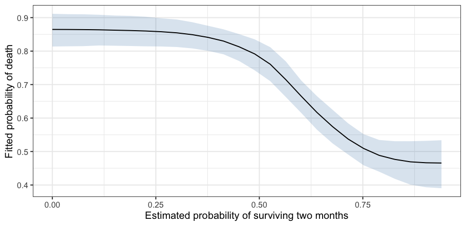
Nothing had to be specified about which predictors matter, which are
curved, or which interact. plot() after partial_dependence() shows
what the model made of one of them, here the study’s own estimate of
each patient’s chance of surviving two months:
partial_dependence(fit, ~ surv2m) |>
  plot() +
  ggplot2::labs(x = "Estimated probability of surviving two months",
                y = "Fitted probability of death")
A forest has no coefficients, so an effect is a contrast between what the model predicts under one value of a predictor and under another, averaged over the sample. Every posterior draw goes through that contrast, so what comes back is a credible interval rather than a standard error:
estimate_effect(fit, treat = "rhc")
#> Average treatment effect (difference)
#>
#> Treatment: `rhc`
#> Averaged over 1500 units
#>
#>     contrast estimate  lower upper    n
#>  Y[1] - Y[0]    0.064 0.0143  0.11 1500
#>
#> Average potential outcomes
#>
#>  quantity estimate lower upper
#>      Y[0]    0.631 0.602 0.659
#>      Y[1]    0.695 0.656 0.732
#>
#> ℹ estimate is the posterior mean; lower and upper bound the 95% equal-tailed
#>   credible interval.
#> ℹ Y[a] is the average response with `rhc` set to "a".
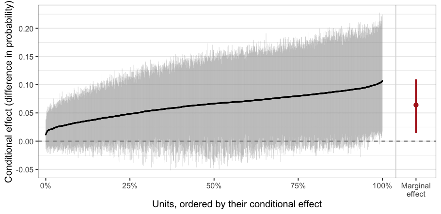
To examine effect heterogeneity, one can generate a plot of conditional effect estimates for all units:
estimate_effect(fit, treat = "rhc", estimand = "CATE") |>
  plot()
Learning More
vignette("bartisan") is the place to start. It carries one analysis
from the formula through to the estimates, and each of its sections
points at the guide that takes that step further:
| Topic | Vignette |
|---|---|
| Choosing a response family | vignette("families") |
| Censored and survival outcomes | vignette("survival") |
| Varying coefficient models | vignette("varying") |
| Effects, curves, and interactions | vignette("effects") |
| Which predictors the model uses | vignette("importance") |
| Convergence and model fit | vignette("diagnostics") |
| Comparing and selecting models | vignette("comparison") |
| Causal inference and Bayesian causal forests | vignette("causal") |
| What the model is and how it is fitted | vignette("implementation") |
| Short answers to common questions | vignette("faq") |
A fitted model also works with the packages that already read Bayesian fits: marginaleffects for a wider range of estimands, loo for model comparison, bayesplot and posterior for the draws themselves, and performance for fit statistics. Load one and call its functions on the fit; there is nothing to set up.
Citing bartisan
bartisan implements the sampler of Linero (2025),
and its MCMC engine is adapted from that paper’s FlexBart reference
implementation. Please cite the method and the package both, the latter
with its version number, which citation("bartisan") supplies. The
smooth decision rules are those of Linero and Yang
(2018). Both papers are listed under References
below.
Questions and Bug Reports
Please file an issue at https://github.com/ngreifer/bartisan/issues, with a reproducible example where the report concerns a fit.
References
Connors, Alfred F., Theodore Speroff, Neal V. Dawson, et al. 1996. “The Effectiveness of Right Heart Catheterization in the Initial Care of Critically Ill Patients.” JAMA 276 (11): 889–97. https://doi.org/10.1001/jama.1996.03540110043030.
Linero, Antonio R. 2025. “Generalized Bayesian Additive Regression Trees Models: Beyond Conditional Conjugacy.” Journal of the American Statistical Association 120 (549): 356–69. https://doi.org/10.1080/01621459.2024.2337156.
Linero, Antonio R., and Yun Yang. 2018. “Bayesian Regression Tree Ensembles That Adapt to Smoothness and Sparsity.” Journal of the Royal Statistical Society Series B: Statistical Methodology 80 (5): 1087–110. https://doi.org/10.1111/rssb.12293.