Bayesian Neural Network with 'Stan'

Offers a flexible formula-based interface for building and training Bayesian Neural Networks powered by 'Stan'. The package supports modeling complex relationships while providing rigorous uncertainty quantification via posterior distributions. With features like user chosen priors, clear predictions, and support for regression, binary, and multi-class classification, it is well-suited for applications in clinical trials, finance, and other fields requiring robust Bayesian inference and decision-making. References: Neal(1996) .

bnns

The bnns package provides tools to fit Bayesian Neural Networks (BNNs) for regression and classification problems. It is designed to be flexible, supporting various network architectures, activation functions, and output types, making it suitable for both simple and complex data analysis tasks.

Features

• Support for multi-layer neural networks with customizable architecture.
• Choice of activation functions (e.g., sigmoid, ReLU, tanh) and output types for regression (continuous) and classification (binary and multiclass).
• Choice of prior distributions for weights, biases and sigma (for regression).
• Seamless integration with the tidymodels ecosystem (parsnip, recipes, workflows, tune).
• GPU acceleration support via OpenCL for significantly faster model training (requires cmdstanr to be installed separately).
• Built-in functions for model evaluation (loo.bnns(), waic.bnns()), plotting (plot.bnns()), and saving/loading (save_bnns(), load_bnns()).
• Bayesian inference, providing rigorous uncertainty quantification via posterior distributions for predictions and parameters.
• Applications in domains such as clinical trials, predictive modeling, and more.

Why bnns instead of brms?

While brms is an exceptionally powerful tool for general Bayesian regression and mixed-effects models, bnns is purpose-built specifically for Bayesian Neural Networks (BNNs). Here is why you might choose bnns for these specific tasks:

• Simplified Architecture Setup: bnns allows you to define complex, multi-layer neural networks intuitively using straightforward arguments (L for number of layers, nodes for nodes per layer, act_fn for activation functions). Implementing a multi-layer feed-forward neural network in brms requires writing extremely complex, custom non-linear formulas.
• Native tidymodels Integration: bnns provides first-class support for the tidymodels ecosystem (parsnip, recipes, tune, workflows). This makes it seamless to incorporate Bayesian Neural Networks into standard R machine learning pipelines, cross-validation, and hyperparameter tuning workflows.
• Purpose-Built Stan Code: The underlying Stan code generated by bnns is tailored explicitly for neural network matrix multiplications and feed-forward passes, keeping model compilation and execution efficient for deep learning structures.
• Out-of-the-Box Classification: Easily handle continuous regression, binary classification, and multi-class classification natively with built-in output activation functions (out_act_fn).

Installation (stable CRAN version)

To install the bnns package from CRAN, use the following:

install.packages("bnns")

Installation (development version)

To install the bnns package from GitHub, use the following:

# Install devtools if not already installed
if (!requireNamespace("devtools", quietly = TRUE)) {
  install.packages("devtools")
}

# Install bnns
devtools::install_github("swarnendu-stat/bnns")

Getting Started

1. Iris Data

We use the iris data for regression:

head(iris)
#>   Sepal.Length Sepal.Width Petal.Length Petal.Width Species
#> 1          5.1         3.5          1.4         0.2  setosa
#> 2          4.9         3.0          1.4         0.2  setosa
#> 3          4.7         3.2          1.3         0.2  setosa
#> 4          4.6         3.1          1.5         0.2  setosa
#> 5          5.0         3.6          1.4         0.2  setosa
#> 6          5.4         3.9          1.7         0.4  setosa

2. Fit a BNN Model

To fit a Bayesian Neural Network:

library(bnns)

iris_bnn <- bnns(Sepal.Length ~ -1 + ., data = iris, L = 1, act_fn = "softplus", nodes = 4, out_act_fn = "linear", chains = 1)

3. Model Summary

Summarize the fitted model:

summary(iris_bnn)
#> Call:
#> bnns.default(formula = Sepal.Length ~ -1 + ., data = iris, L = 1, 
#>     nodes = 4, act_fn = "softplus", out_act_fn = "linear", chains = 1)
#> 
#> Data Summary:
#> Number of observations: 150 
#> Number of features: 6 
#> 
#> Network Architecture:
#> Number of hidden layers: 1 
#> Nodes per layer: 4 
#> Activation functions: 3 
#> Output activation function: 1 
#> 
#> Posterior Summary (Key Parameters):
#>                mean      se_mean         sd        2.5%         25%        50%
#> w_out[1] -0.5942278 0.2183999192 0.79456857 -1.86701355 -1.09251619 -0.8169628
#> w_out[2]  0.8336814 0.1038869956 0.73827166 -0.51846423  0.33211823  0.7957336
#> w_out[3]  0.4338102 0.2921135070 0.86147575 -1.36143601  0.04394916  0.5954254
#> w_out[4]  0.6850131 0.1360689685 0.76972857 -1.04704293  0.29744188  0.7507712
#> b_out[1]  2.2618133 0.0769776211 1.17876734 -0.02391873  1.42283776  2.2881991
#> sigma     0.3020955 0.0005477896 0.01953213  0.26715455  0.28850768  0.3012247
#>                  75%     97.5%       n_eff      Rhat
#> w_out[1] -0.01503725 1.2874762   13.236032 1.0106679
#> w_out[2]  1.24910581 2.3385023   50.502168 0.9987815
#> w_out[3]  1.00906365 1.8752488    8.697268 1.1745061
#> w_out[4]  1.21289586 1.9468606   32.000519 1.0439056
#> b_out[1]  3.13716320 4.3023801  234.491563 1.0087978
#> sigma     0.31349020 0.3406216 1271.368723 0.9999925
#> 
#> Model Fit Information:
#> Iterations: 1000 
#> Warmup: 200 
#> Thinning: 1 
#> Chains: 1 
#> 
#> Predictive Performance:
#> RMSE (training): 0.2820529 
#> MAE (training): 0.2234438 
#> 
#> Notes:
#> Check convergence diagnostics for parameters with high R-hat values.

4. Predictions

Make predictions using the trained model:

pred <- predict(iris_bnn)

5. Visualization

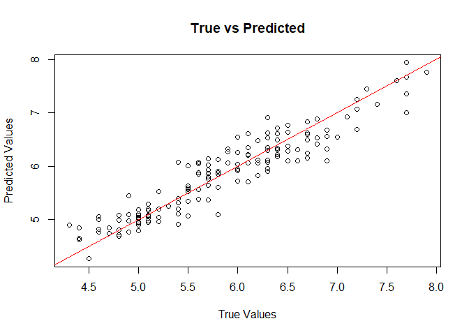
Visualize true vs predicted values for regression:

plot(iris$Sepal.Length, rowMeans(pred), main = "True vs Predicted", xlab = "True Values", ylab = "Predicted Values")
abline(0, 1, col = "red")

Applications

Regression Example (with custom priors)

Use bnns for regression analysis to model continuous outcomes, such as predicting patient biomarkers in clinical trials.

model <- bnns(Sepal.Length ~ -1 + .,
  data = iris, L = 1, act_fn = "softplus", nodes = 4,
  out_act_fn = "linear", chains = 1,
  prior_weights = list(dist = "uniform", params = list(alpha = -1, beta = 1)),
  prior_bias = list(dist = "cauchy", params = list(mu = 0, sigma = 2.5)),
  prior_sigma = list(dist = "inv_gamma", params = list(alpha = 1, beta = 1))
)

Classification Example

For binary or multiclass classification, set the out_act_fn to 2 (binary) or 3 (multiclass). For example:

# Simulate binary classification data
df <- data.frame(
  x1 = runif(10), x2 = runif(10),
  y = sample(0:1, 10, replace = TRUE)
)

# Fit a binary classification BNN
model <- bnns(y ~ -1 + x1 + x2,
  data = df, L = 2, nodes = c(16, 8),
  act_fn = c("softplus", "sigmoid"), out_act_fn = "sigmoid", iter = 1e2,
  warmup = 5e1, chains = 1
)

Clinical Trial Applications

Explore posterior probabilities to estimate treatment effects or success probabilities in clinical trials. For example, calculate the posterior probability of achieving a clinically meaningful outcome in a given population.

Documentation

• Detailed vignettes are available to guide through various applications of the package.
• See help(bnns) for more information about the bnns function and its arguments.

Contributing

Contributions are welcome! Please raise issues or submit pull requests on GitHub.

License

This package is licensed under the MIT License. See LICENSE for details.