campsismod
Generic Implementation of a PK/PD Model
A generic, easy-to-use and expandable implementation of a pharmacokinetic (PK) / pharmacodynamic (PD) model based on the S4 class system. This package allows the user to read and write pharmacometric models from and to files, including a JSON-based interface to import Campsis models defined using a formal JSON schema distributed with the package. Models can be adapted further on the fly in the R environment using an intuitive API to add, modify or delete equations, ordinary differential equations (ODEs), model parameters or compartment properties (such as infusion duration or rate, bioavailability and initial values). The package also provides export facilities for use with the simulation packages 'rxode2' and 'mrgsolve'. The package itself is licensed under the GPL (>= 3); the JSON schema file shipped in inst/extdata is licensed separately under the Creative Commons Attribution 4.0 International (CC BY 4.0). This package is designed and intended to be used with the package 'campsis', a PK/PD simulation platform built on top of 'rxode2' and 'mrgsolve'.
campsismod 


Installation
You can install the released version of campsismod from CRAN with:
install.packages("campsismod")
Alternatively, the package can also be installed with devtools:
devtools::install_github("Calvagone/campsismod")
Basic examples
Load example from model library
Load 2-compartment PK model from built-in model library:
library(campsismod)
model <- model_suite$pk$`2cpt_fo`
Write Campsis model
The model can be exported to files using write.
model %>% write(file = "path_to_model_folder")
In this case, the model code will be contained in the model.campsis
file. Parameters (THETA, OMEGA and SIGMA) will be stored in their
respective CSV file.
list.files("path_to_model_folder")
#> [1] "model.campsis" "omega.csv"     "sigma.csv"     "theta.csv"
Alternatively, the model can also be exported in JSON format into a single file:
model %>% write(file = "my_model.json")
Read and show Campsis model
The model can be loaded from the previously created folder:
model <- read.campsis(file = "path_to_model_folder")
Or, from the previously created JSON file:
model <- read.campsis(file = "my_model.json")
The model can then be output in the console using show:
show(model)
#> [MAIN]
#> TVBIO=THETA_BIO
#> TVKA=THETA_KA
#> TVVC=THETA_VC
#> TVVP=THETA_VP
#> TVQ=THETA_Q
#> TVCL=THETA_CL
#>
#> BIO=TVBIO
#> KA=TVKA * exp(ETA_KA)
#> VC=TVVC * exp(ETA_VC)
#> VP=TVVP * exp(ETA_VP)
#> Q=TVQ * exp(ETA_Q)
#> CL=TVCL * exp(ETA_CL)
#>
#> [ODE]
#> d/dt(A_ABS)=-KA*A_ABS
#> d/dt(A_CENTRAL)=KA*A_ABS + Q/VP*A_PERIPHERAL - Q/VC*A_CENTRAL - CL/VC*A_CENTRAL
#> d/dt(A_PERIPHERAL)=Q/VC*A_CENTRAL - Q/VP*A_PERIPHERAL
#>
#> [F]
#> A_ABS=BIO
#>
#> [ERROR]
#> CONC=A_CENTRAL/VC
#> if (CONC <= 0.001) CONC=0.001
#> CONC_ERR=CONC*(1 + EPS_PROP_RUV)
#>
#>
#> THETA's:
#>   name index value   fix                            label unit
#> 1  BIO     1     1 FALSE                  Bioavailability <NA>
#> 2   KA     2     1 FALSE                  Absorption rate  1/h
#> 3   VC     3    10 FALSE    Volume of central compartment    L
#> 4   VP     4    40 FALSE Volume of peripheral compartment    L
#> 5    Q     5    20 FALSE           Inter-compartment flow  L/h
#> 6   CL     6     3 FALSE                        Clearance  L/h
#> OMEGA's:
#>   name index index2 value   fix type
#> 1   KA     1      1    25 FALSE  cv%
#> 2   VC     2      2    25 FALSE  cv%
#> 3   VP     3      3    25 FALSE  cv%
#> 4    Q     4      4    25 FALSE  cv%
#> 5   CL     5      5    25 FALSE  cv%
#> SIGMA's:
#>       name index index2 value   fix type
#> 1 PROP_RUV     1      1   0.1 FALSE   sd
#> No variance-covariance matrix
#>
#> Compartments:
#> A_ABS (CMT=1)
#> A_CENTRAL (CMT=2)
#> A_PERIPHERAL (CMT=3)
Simulate with rxode2 or mrgsolve
library(campsis)

dataset <- Dataset(5) %>%
  add(Bolus(time = 0, amount = 1000, ii = 12, addl = 2)) %>%
  add(Observations(times = 0:36))

rxode <- simulate(model = model, dataset = dataset, dest = "rxode2", seed = 0)
mrgsolve <- simulate(model = model, dataset = dataset, dest = "mrgsolve", seed = 0)
spaghetti_plot(rxode, "CONC")
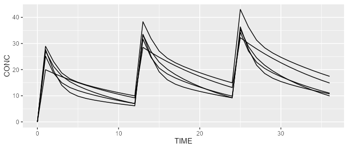 rxode2 simulation results
spaghetti_plot(mrgsolve, "CONC")
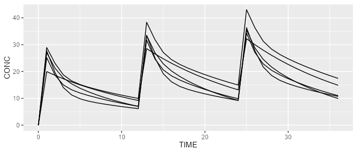 mrgsolve simulation results