Multi-Seasonal ARIMA Models

Fit, forecast and simulate autoregressive integrated moving average (ARIMA) models with more than one seasonal component, following Lisi and Grigoletto (2025) . Series observed at high frequency often display several seasonal cycles at once, such as the daily and the weekly pattern of hourly data, which a single seasonal ARIMA operator cannot represent. Estimation is performed by conditional maximum likelihood through numerical optimisation, with support for fixed coefficients and a constant term. Multi-seasonal Ljung-Box and Monti portmanteau tests, following Grigoletto and Lisi (2026) , seasonal correlograms, forecasts with prediction intervals, and simulation from a model specification or from a fitted model are also provided.

msarima

The msarima package fits ARIMA models with more than one seasonal component. Series observed at high frequency often carry several cycles at once, such as the daily and the weekly pattern of hourly data, while stats::arima() can only take one of them. The package gives each period its own autoregressive, differencing and moving average operator, estimated by conditional maximum likelihood.

• msarima() fits the model, with support for fixed coefficients and a constant term.
• forecast() produces point forecasts and prediction intervals.
• msarima.sim() and simulate() simulate from a specification or from a fit.
• sacf() and spacf() draw correlograms that mark the lags of each cycle (ggsacf() and ggspacf() for the ggplot2 versions).
• msportmanteau() runs the multi-seasonal Ljung-Box and Monti portmanteau tests on a series or on the residuals of a fit.

Installation

You can install the stable version from CRAN:

install.packages("msarima")

You can install the development version from GitHub:

# install.packages("devtools")
devtools::install_github("danigiro/msarima")

Usage

MAD_m40 is the hourly number of vehicles recorded by a sensor on the M-40 ring road of Madrid over the eight weeks from 3 February to 29 March 2024. It is an msts object with periods 24 and 168, so the periods do not have to be repeated in every call.

library(msarima)

plot(window(MAD_m40, end = 4), ylab = "vehicles per hour",
     main = "M-40, first four weeks (time in weeks)")

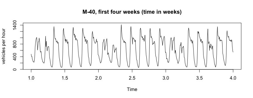
Both the daily cycle and the weekly one (weekends clearly lower) are visible. order sets the non-seasonal part, seasonal takes one c(P, D, Q) per period:

fit <- msarima(MAD_m40,
               order = c(1, 0, 2),
               seasonal = list(c(0, 1, 1), c(0, 1, 1)))
fit
#> Series: MAD_m40 
#> mSARIMA(1,0,2)(0,1,1)[24](0,1,1)[168]
#> 
#> Coefficients:
#>    AR(1)    MA(1)    MA(2) SMA(1,1) SMA(2,1) 
#>   0.8847  -0.3737  -0.0906  -0.5603  -0.6836 
#> 
#> sigma^2 = 4009.7288  log likelihood = -5356.48
#> AIC = 10724.97   AICc = 10725.04   BIC = 10755.26

summary() adds standard errors and significance tests:

summary(fit)
#> Series: MAD_m40 
#> mSARIMA(1,0,2)(0,1,1)[24](0,1,1)[168]
#> 
#> Coefficients:
#>          Estimate Std. Error z value Pr(>|z|)    
#> AR(1)     0.88473    0.02473  35.770   <2e-16 ***
#> MA(1)    -0.37373    0.04060  -9.204   <2e-16 ***
#> MA(2)    -0.09059    0.03805  -2.381   0.0173 *  
#> SMA(1,1) -0.56029    0.02700 -20.748   <2e-16 ***
#> SMA(2,1) -0.68362    0.02525 -27.072   <2e-16 ***
#> ---
#> Signif. codes:  0 '***' 0.001 '**' 0.01 '*' 0.05 '.' 0.1 ' ' 1
#> 
#> sigma^2 = 4009.7288  log likelihood = -5356.4828
#> AIC = 10724.9656   AICc = 10725.0390   BIC = 10755.2612

Forecasting

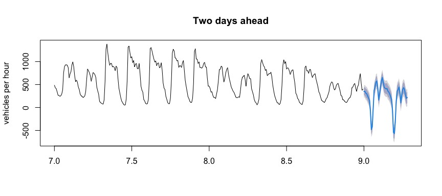
fc <- forecast(fit, h = 48)
plot(fc, include = 336, main = "Two days ahead", ylab = "vehicles per hour")

Simulation

set.seed(1)
y <- msarima.sim(nsim = 500,
                 order = c(1, 0, 1),
                 seasonal = list(c(0, 0, 1), c(0, 0, 1)),
                 seasonal.period = c(7, 30),
                 ar = 0.6, ma = c(0.4, 0.3, 0.2),
                 sigma2 = 0.5)

y_sim <- simulate(fit, nsim = 168, seed = 1)

Fixing parameters

fixed takes one entry per parameter, NA where the parameter is to be estimated. The order is AR, seasonal AR, MA, seasonal MA, sigma:

fit_fixed <- msarima(MAD_m40,
                     order = c(1, 0, 2),
                     seasonal = list(c(0, 1, 1), c(0, 1, 1)),
                     fixed = c(NA, NA, NA, -0.6, NA, NA))
c(free = AIC(fit), fixed = AIC(fit_fixed))
#>     free    fixed 
#> 10724.97 10725.21

Learn more

vignette("msarima") walks through the package on MAD_m40, from the correlograms to model choice and forecast evaluation.

References

Lisi, F. and Grigoletto, M. (2025). Multiple seasonal autoregressive integrated moving average models. Journal of Forecasting, 44(6), 2037-2052. https://doi.org/10.1002/for.3283

Grigoletto, M. and Lisi, F. (2026). Portmanteau goodness-of-fit tests in the presence of simple, mixed, and multiple seasonal autocorrelation. arXiv. https://doi.org/10.48550/arXiv.2609.32381