Super Learning with Flexible Formulas

A functional programming based implementation of the super learner algorithm with an emphasis on supporting the use of formulas to specify learners. This approach offers several improvements compared to past implementations including the ability to easily use random-effects specified in formulas (like y ~ (age | strata) + ...) and construction of new learners is as simple as writing and passing a new function. The super learner algorithm was originally described in van der Laan et al. (2007) < https://biostats.bepress.com/ucbbiostat/paper222/>.

{nadir}

nadir (noun): nā-dir

the lowest point.

{nadir} implements the super learner algorithm[^1]. To quote the Guide to SuperLearner[^2] (a previous implementation):

SuperLearner is an algorithm that uses cross-validation to estimate the performance of multiple machine learning models, or the same model with different settings. It then creates an optimal weighted average of those models, aka an “ensemble”, using the test data performance. This approach has been proven to be asymptotically as accurate as the best possible prediction algorithm that is tested.

Fitting with the minimum loss based estimation literature,[^3]^,[^4] {nadir} is an implementation of the super learner algorithm with improved support for flexible formula based syntax and which is fond of functional programming techniques such as closures, currying, and function factories.

Installation Instructions

You may install {nadir} from GitHub by running:

devtools::install_github("ctesta01/nadir")

We expect {nadir} to be available from CRAN soon. Once it is available on CRAN, you may install it from CRAN using

install.packages("nadir")

Why {nadir} and why reimplement super learner again?

In previous implementations ({SuperLearner}, {sl3}, {mlr3superlearner}), support for flexible formula-based syntax has been limited, instead opting for specifying learners as models on an $X$ matrix and $Y$ outcome vector. Many popular R packages such as lme4 and mgcv (for random effects and generalized additive models) use formulas extensively to specify models using syntax like (age | strata) to specify random effects on age by strata, or s(age, income) to specify a smoothing term on age and income simultaneously.

At present, it is difficult to use these kinds of features in {SuperLearner}, {sl3} and {mlr3superlearner}.

For example, it is easy to imagine the super learner algorithm being appealing to modelers fond of random effects based models because they may want to hedge on the exact nature of the random effects models, not sure if random intercepts are enough or if random slopes should be included, etc., and similar other modeling decisions in other frameworks.

Therefore, the {nadir} package takes as its charges to:

• Implement a syntax in which it is easy to specify different formulas for each of many candidate learners.
• To make it easy to pass new learners to the Super Learner algorithm.

Demonstration

First, let’s start with the simplest possible use case of nadir::super_learner(), which is where the user would like to feed in data, a specification for some regression formula(s), specify a library of learners, and get back a prediction function that is suitable for plugging into downstream analyses, like in Targeted Learning or for pure-prediction applications.

Here is a demo of an extremely simple application of using nadir::super_learner:

library(nadir)

# we'll use a few basic learners
learners <- list(
     glm = lnr_glm,
     rf = lnr_rf,
     glmnet = lnr_glmnet
  )
# more learners are available, see ?learners

sl_model <- super_learner(
  data = mtcars,
  formula = mpg ~ cyl + hp + disp,
  learners = learners)

# the output from super_learner is a prediction function:
# here we are producing predictions based on a weighted combination of the
# trained learners. 
predict(sl_model, mtcars) |> head()

##         Mazda RX4     Mazda RX4 Wag        Datsun 710    Hornet 4 Drive 
##          20.41648          20.41648          24.20135          19.85172 
## Hornet Sportabout           Valiant 
##          16.89780          19.59764

One Step Up: Fancy Formula Features

Continuing with our mtcars example, suppose the user would really like to use random effects or similar types of fancy formula language features. One easy way to do so with nadir::super_learner is using the following syntax:

learners <- list(
     glm = lnr_glm,
     rf = lnr_rf,
     glmnet = lnr_glmnet,
     lmer = lnr_lmer,
     gam = lnr_gam
  )

formulas <- c(
  .default = mpg ~ cyl + hp + disp,   # our first three learners use same formula
  lmer = mpg ~ (1 | cyl) + hp + disp, # both lme4::lmer and mgcv::gam have 
  gam = mpg ~ s(hp) + cyl + disp      # specialized formula syntax
  )

# fit a super_learner
sl_model <- super_learner(
  data = mtcars,
  formulas = formulas,
  learners = learners)
  
predict(sl_model, mtcars) |> head()

##         Mazda RX4     Mazda RX4 Wag        Datsun 710    Hornet 4 Drive 
##          20.53980          20.53980          24.43141          19.74459 
## Hornet Sportabout           Valiant 
##          16.82782          19.64837

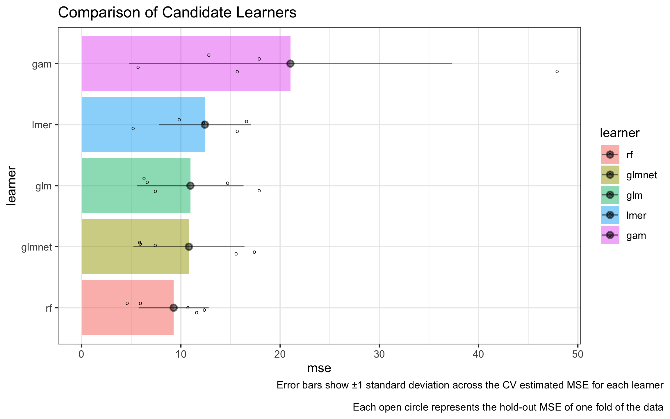
How should we assess performance of nadir::super_learner()?

To put the learners and the super learner algorithm on a level playing field, it’s important that learners and super learner both be evaluated on held-out validation/test data that the algorithms have not seen before.

Using the output from nadir::super_learner(), we can call compare_learners() to see the mean-squared-error (MSE) on the held-out data, also called CV-MSE, for each of the candidate learners specified.

# construct our super learner and call compare_learners on it
sl_model <- super_learner(
  data = mtcars,
  formulas = formulas,
  learners = learners)
  
compare_learners(sl_model)

## Inferring the loss metric for learner comparison based on the outcome type:

## outcome_type=continuous -> using mean squared error

## # A tibble: 1 × 5
##     glm    rf glmnet  lmer   gam
##   <dbl> <dbl>  <dbl> <dbl> <dbl>
## 1  10.8  7.25   10.9  9.44  10.9

Plotting code

pacman::p_load('dplyr', 'ggplot2', 'tidyr', 'magrittr')

truth <- sl_model$holdout_predictions$mpg

holdout_var <- sl_model$holdout_predictions |>
  dplyr::group_by(.sl_fold) |> 
  dplyr::summarize(across(everything(), ~ mean((. - mpg)^2))) |> 
  dplyr::summarize(across(everything(), var)) |> 
  select(-mpg, -.sl_fold) |> 
  t() |> 
  as.data.frame() |> 
  tibble::rownames_to_column('learner') |> 
  dplyr::rename(var = V1) |>
  dplyr::mutate(sd = sqrt(var))


jitters <- sl_model$holdout_predictions |> 
  dplyr::mutate(dplyr::across(-.sl_fold, ~ (. - mpg)^2)) |> 
  dplyr::select(-mpg) %>%
  tidyr::pivot_longer(cols = 2:ncol(.), names_to = 'learner', values_to = 'squared_error') |>
  dplyr::group_by(learner, .sl_fold) |> 
  dplyr::summarize(mse = mean(squared_error)) |> 
  ungroup() |> 
  rename(fold = .sl_fold)

## `summarise()` has grouped output by 'learner'. You can override using the
## `.groups` argument.

learner_comparison_df <- sl_model |> 
  compare_learners() |> 
  t() |> 
  as.data.frame() |>
  tibble::rownames_to_column(var = 'learner') |> 
  dplyr::mutate(learner = factor(learner)) |>
  dplyr::rename(mse = V1) |>
  dplyr::left_join(holdout_var) |> 
  dplyr::mutate(
    upper_ci = mse + sd,
    lower_ci = mse - sd) |> 
  dplyr::mutate(learner = forcats::fct_reorder(learner, mse))

## Inferring the loss metric for learner comparison based on the outcome type: 
## outcome_type=continuous -> using mean squared error
## Joining with `by = join_by(learner)`

jitters$learner <- factor(jitters$learner, levels = levels(learner_comparison_df$learner))

learner_comparison_df |> 
  ggplot2::ggplot(ggplot2::aes(y = learner, x = mse, fill = learner)) + 
  ggplot2::geom_col(alpha = 0.5) + 
  ggplot2::geom_jitter(data = jitters, mapping = ggplot2::aes(x = mse), height = .15, shape = 'o') + 
  ggplot2::geom_pointrange(mapping = ggplot2::aes(xmax = upper_ci, xmin = lower_ci),
                           alpha = 0.5) + 
  ggplot2::theme_bw() + 
  ggplot2::ggtitle("Comparison of Candidate Learners") + 
  ggplot2::labs(caption = "Error bars show ±1 standard deviation across the CV estimated MSE for each learner\n
Each open circle represents the hold-out MSE of one fold of the data") + 
  ggplot2::theme(plot.caption.position = 'plot')

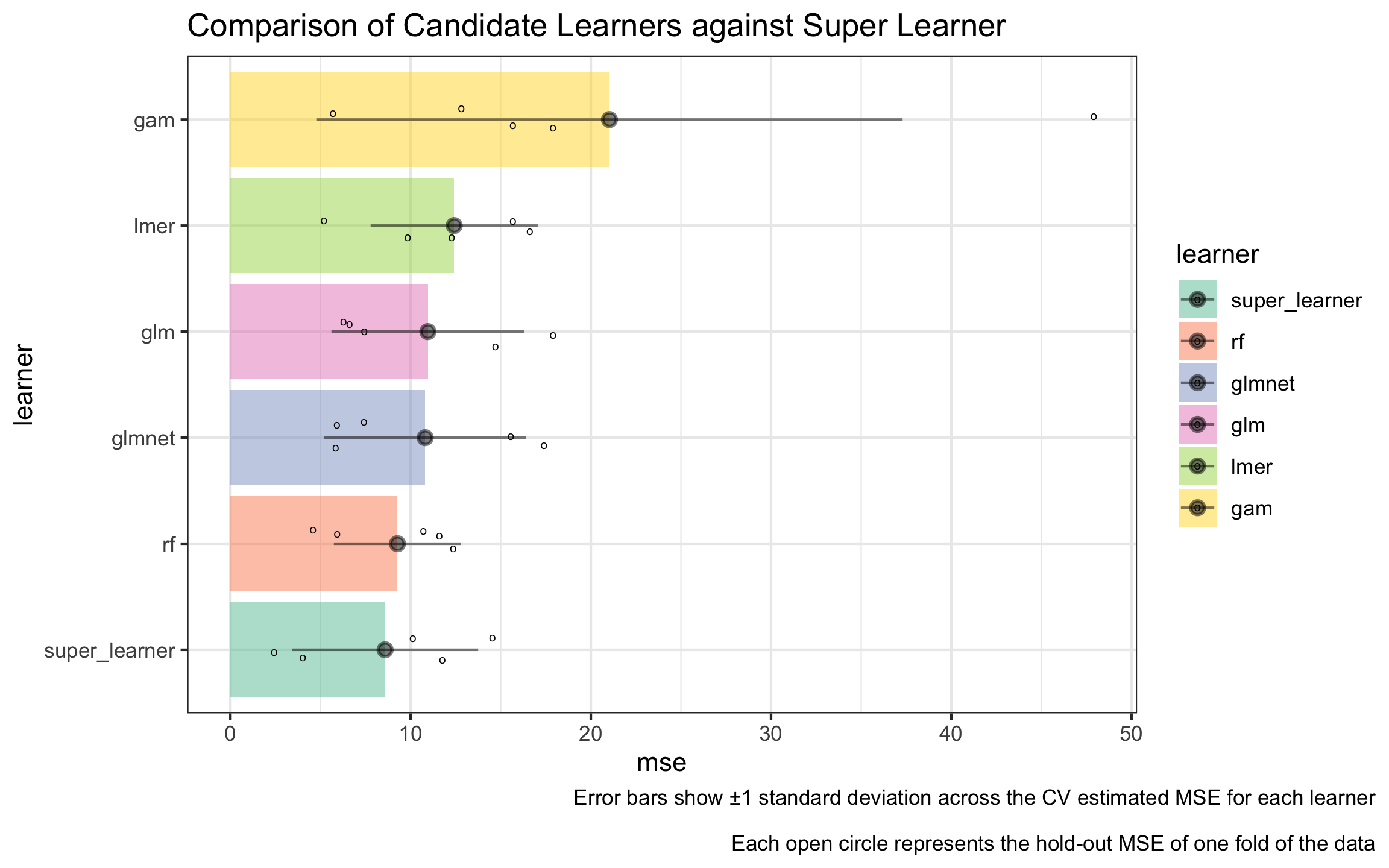
Now how should we go about getting the CV-MSE from a super learned model? We will use the cv_super_learner() function that performs another layer of cross-validation in order to assess the specified super learner on folds of held-out data.

If you’d like to read more about how the internals of cv_super_learner() work, please refer to the article Currying, Closures, and Function Factories article

cv_results <- cv_super_learner(
  data = mtcars,
  formulas = formulas,
  learners = learners)

cv_results

## $cv_trained_learners
## # A tibble: 5 × 4
##   split learned_predictor predictions mpg      
##   <int> <list>            <list>      <list>   
## 1     1 <fn>              <dbl [6]>   <dbl [6]>
## 2     2 <fn>              <dbl [7]>   <dbl [7]>
## 3     3 <fn>              <dbl [6]>   <dbl [6]>
## 4     4 <fn>              <dbl [6]>   <dbl [6]>
## 5     5 <fn>              <dbl [7]>   <dbl [7]>
## 
## $cv_loss
## [1] 7.337934

Plotting code

cv_jitters <- cv_results$cv_trained_learners |> 
  dplyr::select(split, predictions, mpg) |> 
  tidyr::unnest(cols = c('predictions', 'mpg')) |> 
  dplyr::group_by(split) |> 
  dplyr::summarize(mse = mean((mpg - predictions)^2)) |>
  dplyr::bind_cols(learner = 'super_learner')


cv_var <- cv_results$cv_trained_learners |> 
  dplyr::select(split, predictions, mpg) |> 
  tidyr::unnest(cols = c(predictions, mpg)) |> 
  dplyr::mutate(squared_error = (mpg - predictions)^2) |> 
  dplyr::group_by(split) |> 
  dplyr::summarize(mse = mean(squared_error)) |> 
  dplyr::summarize(
    var = var(mse),
    mse = mean(mse),
    sd = sqrt(var),
    upper_ci = mse + sd,
    lower_ci = mse - sd) |> 
  dplyr::bind_cols(learner = 'super_learner')

new_jitters <- bind_rows(jitters, cv_jitters)

learner_comparison_df |> 
  bind_rows(cv_var) |> 
  dplyr::mutate(learner = forcats::fct_reorder(learner, mse)) |> 
  ggplot2::ggplot(ggplot2::aes(y = learner, x = mse, fill = learner)) + 
  ggplot2::geom_col(alpha = 0.5) + 
  ggplot2::geom_jitter(data = new_jitters, mapping = ggplot2::aes(x = mse), height = .15, shape = 'o') + 
  ggplot2::geom_pointrange(mapping = ggplot2::aes(xmax = upper_ci, xmin = lower_ci),
                           alpha = 0.5) + 
  ggplot2::theme_bw() + 
  ggplot2::scale_fill_brewer(palette = 'Set2') + 
  ggplot2::ggtitle("Comparison of Candidate Learners against Super Learner") + 
  ggplot2::labs(caption = "Error bars show ±1 standard deviation across the CV estimated MSE for each learner\n
Each open circle represents the hold-out MSE of one fold of the data") + 
  ggplot2::theme(plot.caption.position = 'plot')

What about model hyperparameters or extra arguments?

Model hyperparameters are easy to handle in {nadir}. Two easy solutions are available to users:

• nadir::super_learner() has an extra_learner_args parameter that can be passed a list of extra arguments for each learner.
• Users can always build new learners (which allows for building in the hyperparameter specification), and using the ... syntax, it’s easy to build new learners from the learners already provided by {nadir}.

Here’s some examples showing each approach.

Using extra_learner_args:

# when using extra_learner_args, it's totally okay to use the 
# same learner multiple times as long as their hyperparameters differ.

sl_model <- nadir::super_learner(
  data = mtcars,
  formula = mpg ~ .,
  learners = c(
    glmnet0 = lnr_glmnet,
    glmnet1 = lnr_glmnet,
    glmnet2 = lnr_glmnet,
    rf0 = lnr_rf,
    rf1 = lnr_rf,
    rf2 = lnr_rf
    ),
  extra_learner_args = list(
    glmnet0 = list(lambda = 0.01),
    glmnet1 = list(lambda = 0.1),
    glmnet2 = list(lambda = 1),
    rf0 = list(ntree = 3),
    rf1 = list(ntree = 10),
    rf2 = list(ntree = 30)
    )
)

compare_learners(sl_model)

## Inferring the loss metric for learner comparison based on the outcome type:

## outcome_type=continuous -> using mean squared error

## # A tibble: 1 × 6
##   glmnet0 glmnet1 glmnet2   rf0   rf1   rf2
##     <dbl>   <dbl>   <dbl> <dbl> <dbl> <dbl>
## 1    11.7    8.69    8.94  10.1  7.00  5.77

Building New Learners Programmatically

When does it make more sense to build new learners with the hyperparameters built into them rather than using the extra_learner_args parameter?

One instance when building new learners may make sense is when the user would like to produce a large number of hyperparameterized learners programmatically, for example over a grid of hyperparameter values. Below we show such an example for a 1-d grid of hyperparameters with glmnet.

# produce a "grid" of glmnet learners with lambda set to 
# exp(-1 to 1 in steps of .1)
hyperparameterized_learners <- lapply(
  exp(seq(-1, 1, by = .1)),
  function(lambda) { 
    # create a new learner with given lambda
    new_learner <- function(data, formula, ...) {
        lnr_glmnet(data, formula, lambda = lambda, ...) }
    
    # declare it to be a continuous outcome learner
    attr(new_learner, 'sl_lnr_type') <- 'continuous'
    
    return(new_learner)
  }
)
  
# give them names because nadir::super_learner requires that the 
# learners argument be named.
names(hyperparameterized_learners) <- paste0('glmnet', 1:length(hyperparameterized_learners))

# fit the super_learner with 20 glmnets with different lambdas
sl_model_glmnet <- nadir::super_learner(
  data = mtcars,
  learners = hyperparameterized_learners,
  formula = mpg ~ .)

compare_learners(sl_model_glmnet)

## Inferring the loss metric for learner comparison based on the outcome type:

## outcome_type=continuous -> using mean squared error

## # A tibble: 1 × 21
##   glmnet1 glmnet2 glmnet3 glmnet4 glmnet5 glmnet6 glmnet7 glmnet8 glmnet9
##     <dbl>   <dbl>   <dbl>   <dbl>   <dbl>   <dbl>   <dbl>   <dbl>   <dbl>
## 1    10.0    9.85    9.57    9.31    9.05    8.76    8.49    8.25    8.05
## # ℹ 12 more variables: glmnet10 <dbl>, glmnet11 <dbl>, glmnet12 <dbl>,
## #   glmnet13 <dbl>, glmnet14 <dbl>, glmnet15 <dbl>, glmnet16 <dbl>,
## #   glmnet17 <dbl>, glmnet18 <dbl>, glmnet19 <dbl>, glmnet20 <dbl>,
## #   glmnet21 <dbl>

What are currying, closures, and function factories?

R is a functional programming language, which allows for functions to build and return functions just like any other return object.

We refer to functions that create and return another function as a function factory. For an extended reference, see the Advanced R book.

Function factories are so useful in {nadir} because, at their essence, a candidate learner needs to be able to 1) accept training data, and 2) produce a prediction function that can make predictions on heldout validation data. So a typical learner in {nadir} looks like:

lnr_lm <- function(data, formula, ...) {
  model <- stats::lm(formula = formula, data = data, ...)

  predict_from_trained_lm <- function(newdata) {
    predict(model, newdata = newdata, type = 'response')
  }
  return(predict_from_trained_lm)
}

Moreover, given how code-lightweight it is to write a simple learner, this makes it relatively easy for users to write new learners that meet their exact needs.

If you want to implement your own learners, you just need to follow the following pseudocode approach:

lnr_custom <- function(data, formula, ...) {
  model <- # train your model using data, formula, ... 
  
  predict_from_model <- function(newdata) {
    return(...) # return predictions from the trained model 
    # (predictions should be a vector of predictions, one for each row of newdata)
  }
  return(predict_from_model)
}

For more details, read the Currying, Closures, and Function Factories article

What all can super_learner() do?

There is built-in support for

• Binary and multiclass outcomes
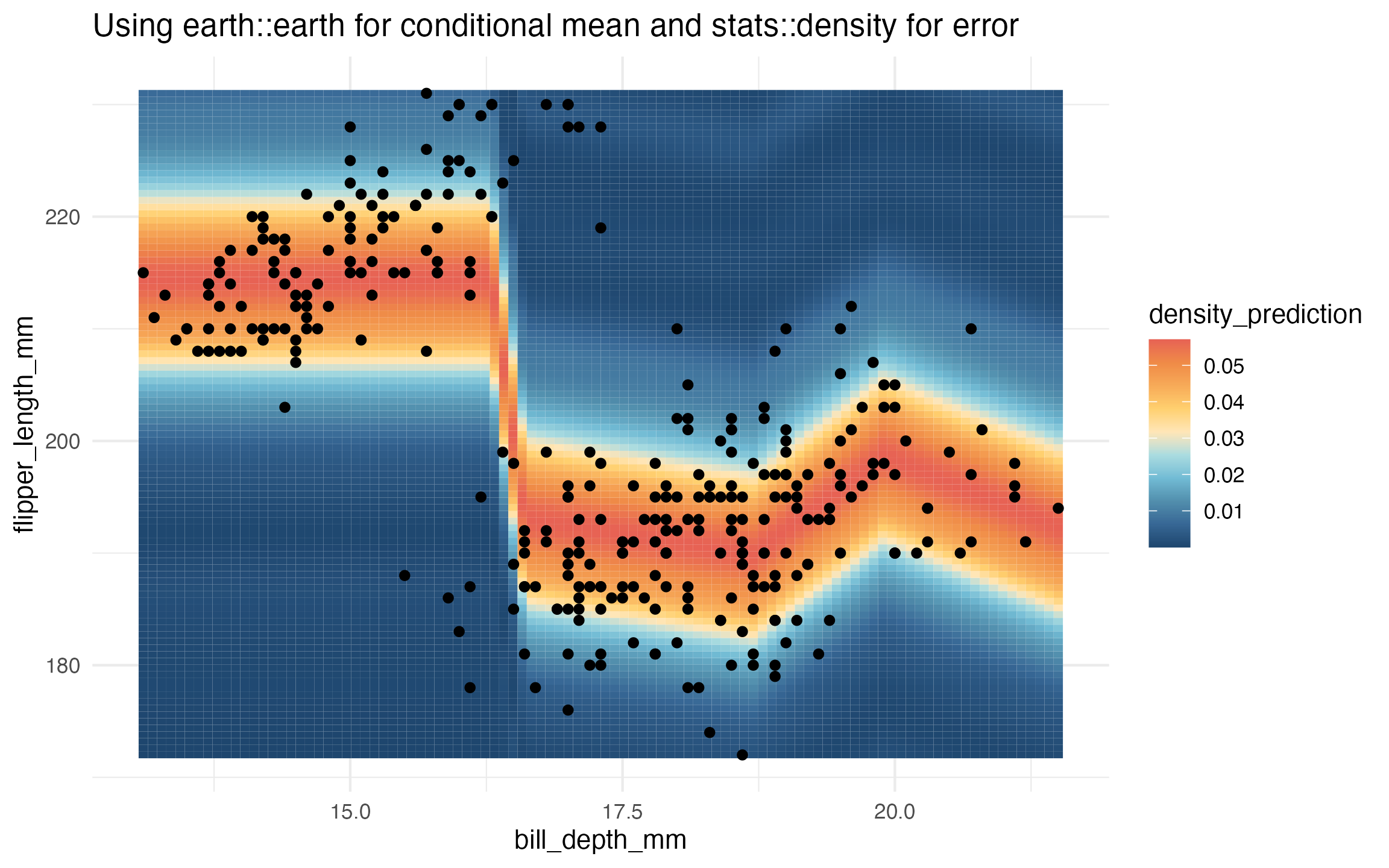
• Density estimation
• Using observation weights
• Running super_learner() in parallel
• Graceful error handling
• Survival analysis via pooled logistic regression
• Working with clusters and strata

As a teaser, here’s an example visualization of a density learner trained on the penguins data:

We also have ≥34 tests (and counting!) that are run at every update to ensure the correctness of the implementation.

View the source code for the tests that are part of {nadir}:

• https://github.com/ctesta01/nadir/tree/main/tests/testthat

Check out the complete documentation on the package website:

• https://ctesta01.github.io/nadir/

Coming Down the Pipe ↩️🚰🔧✨

• (Even More) Automated tests that try to ensure validity/correctness of the implementation!
• Expanding the library of built-in learners
• We may extend to time-series and more outcome types in the future!
• Check out our Feature Requests and Issue Tracker for more

[^1]: van der Laan, M. J., Polley, E. C., & Hubbard, A. E. (2007). Super Learner. In Statistical Applications in Genetics and Molecular Biology (Vol. 6, Issue 1). Walter de Gruyter GmbH. https://doi.org/10.2202/1544-6115.1309 https://pubmed.ncbi.nlm.nih.gov/17910531/

[^2]: Guide to {SuperLearner}: https://cran.r-project.org/package=SuperLearner

[^3]: van der Laan, Mark J. and Dudoit, Sandrine, “Unified Cross-Validation Methodology For Selection Among Estimators and a General Cross-Validated Adaptive Epsilon-Net Estimator: Finite Sample Oracle Inequalities and Examples” (November 2003). U.C. Berkeley Division of Biostatistics Working Paper Series. Working Paper 130. https://biostats.bepress.com/ucbbiostat/paper130/

[^4]: Zheng, W., & van der Laan, M. J. (2011). Cross-Validated Targeted Minimum-Loss-Based Estimation. In Springer Series in Statistics (pp. 459–474). Springer New York. https://doi.org/10.1007/978-1-4419-9782-1_27